Pseudo-spectral derivative of quadratic quasi-interpolant splines

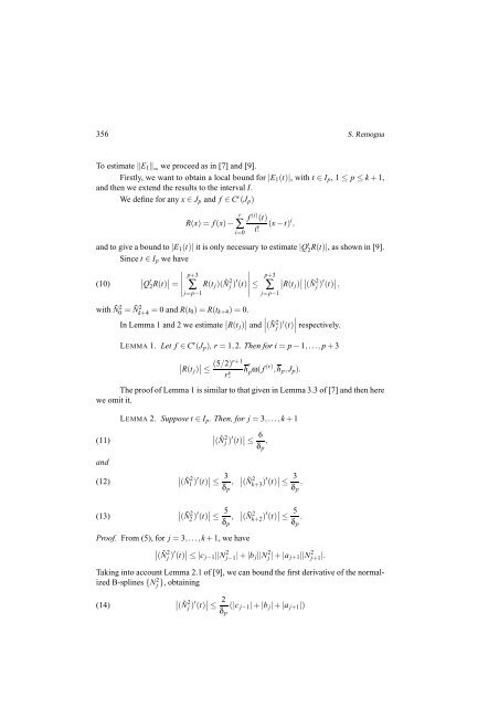
356 S. Remogna
To estimate‖E 1 ‖ ∞ we proceed as in [7] and [9].
Firstly, we want to obtain a local bound for |E 1 (t)|, with t ∈ I p , 1≤ p≤k+ 1,
and then we extend the results to the interval I.
We define for any x∈J p and f ∈ C r (J p )
R(x)= f(x)−
r
∑
i=0
f (i) (t)
(x− t) i ,
i!
and to give a bound to|E 1 (t)| it is only necessary to estimate|Q ′ 2R(t)|, as shown in [9].
Since t ∈ I p we have
(10)
∣ Q
′
2 R(t) ∣ ∣ ∣∣∣∣ p+3
= ∑ R(t j )(Ñ 2 p+3
j )′ (t)
∣ ≤ ∑
j=p−1
j=p−1
∣ R(t j ) ∣ ∣ ∣ ∣ (Ñ 2 j )′ (t) ∣ ∣ ,
with Ñ0 2 = Ñ2 k+4 = 0 and R(t 0)=R(t k+4 )=0.
In Lemma 1 and 2 we estimate ∣ R(t j ) ∣ ∣ ∣∣(Ñ and 2 j )′ (t) ∣ respectively.
LEMMA 1. Let f ∈ C r (J p ), r=1,2. Then for i= p−1,..., p+3
∣ R(t j ) ∣ (5/2) r+1
≤ h r p
r!
ω( f(r) ,h p ,J p ).
The proof of Lemma 1 is similar to that given in Lemma 3.3 of [7] and then here
we omit it.
(11)
and
(12)
(13)
LEMMA 2. Suppose t ∈ I p . Then, for j = 3,...,k+1
∣ (Ñ 2 1 )′ (t) ∣ ∣ ≤
3
δ p
,
∣ (Ñ 2 2 )′ (t) ∣ ∣ ≤
5
δ p
,
∣ (Ñ 2 j )′ (t) ∣ ∣ ≤
6
δ p
,
∣ (Ñ 2 k+3 )′ (t) ∣ ∣ ≤
3
δ p
,
∣ (Ñ 2 k+2 )′ (t) ∣ ∣ ≤
5
δ p
.
Proof. From (5), for j = 3,...,k+1, we have
∣ (Ñ 2 j) ′ (t) ∣ ∣ ≤|c j−1 ||N 2 j−1|+|b j ||N 2 j|+|a j+1 ||N 2 j+1|.
Taking into account Lemma 2.1 of [9], we can bound the first derivative of the normalized
B-splines{N 2 j }, obtaining
(14)
∣
∣(Ñ 2 j )′ (t) ∣ ∣≤ 2 δ p
(|c j−1 |+|b j |+|a j+1 |)