DeepXcav Theory Manual
DeepXcav Theory Manual
DeepXcav Theory Manual

Create successful ePaper yourself
Turn your PDF publications into a flip-book with our unique Google optimized e-Paper software.
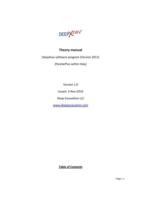
<strong>Theory</strong> manual<br />
<strong>DeepXcav</strong> software program (Version 2011)<br />
(ParatiePlus within Italy)<br />
Version 1.0<br />
Issued: 3-Nov-2010<br />
Deep Excavation LLC<br />
www.deepexcavation.com<br />
Table of Contents<br />
Page | 1
Section Title Page<br />
1 Introduction 4<br />
2 General Analysis Methods 4<br />
3 Ground water analysis methods 4<br />
4 Undrained-Drained Analysis for clays 5<br />
5 Active and Passive Coefficients of Lateral Earth Pressures 5<br />
5.1 Active and Passive Lateral Earth Pressures in Conventional<br />
6<br />
Analyses<br />
5.2 Active and Passive Lateral Earth Pressures in PARATIE module 6<br />
5.3 Passive Pressure Equations 11<br />
5.4 Classical Earth Pressure Options 12<br />
5.4.1 Active & Passive Pressures for non-Level Ground 12<br />
5.4.2 Peck 1969 Earth Pressure Envelopes 14<br />
5.4.3 FHWA Apparent Earth Pressures 15<br />
5.4.4 FHWA Recommended Apparent Earth Pressure Diagram for<br />
17<br />
Soft to Medium Clays<br />
5.4.5 FHWA Loading for Stratified Soil Profiles 17<br />
5.4.6 Modifications to stiff clay and FHWA diagrams 20<br />
5.4.7 Verification Example for Soft Clay and FHWA Approach 24<br />
5.4.8 Custom Trapezoidal Pressure Diagrams 27<br />
5.4.9 Two Step Rectangular Pressure Diagrams 27<br />
5.5 Vertical wall adhesion in undrained loading 29<br />
6 Eurocode 7 analysis methods 30<br />
6.1 Safety Parameters for Ultimate Limit State Combinations 31<br />
6.2 Automatic generation of active and passive lateral earth<br />
38<br />
pressure factors in EC7 type approaches.<br />
6.3 Determination of Water Pressures & Net Water Pressure<br />
39<br />
Actions in the new software (Conventional Limit Equilibrium<br />
Analysis)<br />
6.4 Surcharges 40<br />
6.5 Line Load Surcharges 41<br />
6.6 Strip Surcharges 44<br />
6.7 Other 3D surcharge loads 44<br />
7 Analysis Example with EC7 47<br />
8 Ground anchor and helical anchor capacity calculations<br />
66<br />
Ground Anchor Capacity Calculations<br />
8.1 Ground Anchor Capacity Calculations 66<br />
8.2 Helical anchor capacity calculations 73<br />
Section Title Page<br />
9 Geotechnical Safety Factors 77<br />
Page | 2
9.1 Introduction 77<br />
9.1.1 Introduction 77<br />
9.1.2 Cantilever Walls (conventional analysis) 78<br />
9.1.3 Walls supported by a single bracing level in conventional<br />
79<br />
analyses.<br />
9.1.4 Walls supported by a multiple bracing levels (conventional<br />
79<br />
analysis)<br />
9.2 Clough Predictions & Basal Stability Index 80<br />
9.3 Ground surface settlement estimation 82<br />
10 Handling unbalanced water pressures in Paratie 84<br />
11 Wall Types - Stiffness and Capacity Calculations 85<br />
12 Seismic Pressure Options 89<br />
12.1 Selection of base acceleration and site effects 90<br />
12.2 Determination of retaining structure response factor R 91<br />
12.3 Seismic Thrust Options 93<br />
12.3.1 Semirigid pressure method 94<br />
12.3.2 Mononobe-Okabe 95<br />
12.3.3 Richards Shi method 96<br />
12.3.4 User specified external 97<br />
12.3.5 Wood Automatic method 98<br />
12.3.6 Wood <strong>Manual</strong> 99<br />
12.4 Water Behavior during earthquakes 99<br />
12.5 Wall Inertia Seismic Effects 100<br />
12.6 Verification Example 101<br />
13 Verification of free earth method for a 10ft cantilever<br />
106<br />
excavation<br />
14 Verification of 20 ft deep single-level-supported excavation 111<br />
15 Verification of 30 ft excavation with two support levels 116<br />
Appendix A<br />
Appendix B<br />
APPENDIX: Verification of Passive Pressure Coefficient<br />
Calculations<br />
APPENDIX: Sample Paratie Input File Generated by New<br />
Software Program<br />
120<br />
124<br />
Page | 3
1. Introduction<br />
This document briefly introduces the new <strong>DeepXcav</strong>-Paratie combined software features, analysis<br />
methods, and theoretical background. The handling of Eurocode 7 is emphasized through an<br />
example of a simple single anchor wall.<br />
2. General Analysis Methods<br />
The combined <strong>DeepXcav</strong>-Paratie software is capable of analyzing braced excavations with<br />
“conventional” limit-equilibrium-methods and beam on elastic foundations (i.e. the traditional<br />
PARATIE engine). An excavation can be analyzed in one of the following sequences:<br />
a) Conventional analysis only<br />
b) Paratie analysis only<br />
c) Combined “Conventional”-Paratie Analysis: 1 st Conventional analysis with traditional safety<br />
factors stored in memory. Once the traditional analysis is completed, then the Paratie<br />
analysis is launched.<br />
3. Ground water analysis methods<br />
The software offers the following options for modeling groundwater:<br />
a) Hydrostatic: Applicable for both conventional and Paratie analysis. In Paratie,<br />
hydrostatic conditions are modeled by extending the “wall lining” effect to 100 times the<br />
wall length below the wall bottom.<br />
b) Simplified flow: Applicable for both conventional and Paratie analysis. This is a simplified<br />
1D flow around the wall. In the Paratie analysis mode, the traditional Paratie water flow<br />
option is employed.<br />
c) Full Flow Net analysis: Applicable for both conventional and Paratie analysis. Water<br />
pressures are determined by performing a 2D finite difference flow analysis. In PARATIE,<br />
water pressures are then added by the UTAB command. The flownet analysis does not<br />
account for a drop in the phreatic line.<br />
d) User pressures: Applicable for both conventional and Paratie analysis. Water pressures<br />
defined by the user are assumed. In PARATIE, water pressures are then added by the UTAB<br />
command.<br />
Page | 4
In contrast to PARATIE, conventional analyses do not generate excess pore pressures during<br />
undrained conditions for clays.<br />
4. Undrained-Drained Analysis for clays<br />
Clay behavior depends on the rate of loading (or unloading). When “fast” stress changes take place<br />
then clay behavior is typically modeled as “Undrained” while slow stress changes or long term<br />
conditions are typically modeled as “Drained”.<br />
In the software, the default behavior of a clay type soil is set as “Undrained”. However, the final<br />
Drained/Undrained analysis mode is controlled from the Analysis tab. The software offers the<br />
following Drained/Undrained Analysis Options:<br />
a) Drained: All clays are modeled as drained. In this mode, conventional analysis methods<br />
use the effective cohesion c’ and the effective friction angle φ’ to determine the appropriate<br />
lateral earth pressures. For clays, the PARATIE analysis automatically determines the effective<br />
cohesion from the stress state history and from the peak and constant volume shearing friction<br />
angles (φ peak ’ and φ cv ’ respectively) and it does not use the defined c’ in the soils tab.<br />
b) Undrained: All clays are modeled as undrained. In this mode, conventional analysis methods<br />
use the Undrained Shear Strength S u and assume an effective friction angle φ’=0 o to determine<br />
the appropriate lateral earth pressures. For clays, the PARATIE analysis automatically<br />
determines the Undrained Shear Strength from the stress state history of the clay element and<br />
from the peak and constant volume shearing friction angles (φ peak ’ and φ cv ’ respectively), but<br />
limits the upper S u to the value in the soils tab.<br />
c) Undrained for only initially undrained clays: Only clays whose initial behavior is set to<br />
undrained (Soils form) are modeled as undrained as described in item b) above. All other clays<br />
are modeled as drained.<br />
In contrast to PARATIE, conventional analyses do not generate excess pore pressures during<br />
undrained conditions for clays.<br />
5. Active and Passive Coefficients of Lateral Earth Pressures<br />
The new software offers a number of options for evaluating the “Active” and “Passive” coefficients<br />
that depend on the analysis method employed (Paratie or Conventional). An important difference<br />
with PARATIE is that the old concept of “Uphill” and “Downhill” side has been changed to “Driving<br />
side” and “Resisting Side”. Sections 5.1 and 5.2 present the methods employed in determining active<br />
and passive coefficients/pressures in Conventional and Paratie analyses respectively. However, in all<br />
cases the methods listed in Table 1 available for computing active and passive coefficients.<br />
Page | 5
Table 1: Available Exact Solutions for Active and Passive Lateral Earth Pressure Coefficients<br />
Active Coefficient<br />
Surface<br />
angle<br />
Wall<br />
Friction EQ. 2 Available<br />
Passive Coefficient<br />
Surface<br />
angle<br />
Wall<br />
Friction<br />
Method<br />
Available<br />
Rankine Yes No 1 No 1 No Yes No 1 No 1 No<br />
Coulomb Yes Yes Yes No Yes Yes Yes Yes<br />
Caquot-Kerisel Tabulated No - - - Yes Yes Yes No<br />
Caquot-Kerisel Tabulated No - - - Yes Yes Yes No<br />
Lancellota No - - - Yes Yes Yes Yes<br />
Notes:<br />
1. Rankine method automatically converts to Coulomb if a surface angle or wall friction is included.<br />
2. Seismic effects are added as separately.<br />
EQ.<br />
5.1 Active and Passive Lateral Earth Pressures in Conventional Analyses<br />
In the conventional analysis the software first determines which side is generating driving earth<br />
pressures. Once the driving side is determined, the software examines if a single ground surface<br />
angle is assumed on the driving and on the resisting sides. If a single surface angle is used then the<br />
exact theoretical equation is employed as outlined in. If an irregular ground surface angle is<br />
detected then the program starts performing a wedge analysis on the appropriate side. Horizontal<br />
ground earth pressures are then prorated to account for all applicable effects including wall<br />
friction. It should be noted that the active/passive wedge analyses can take into account flownet<br />
water pressures if a flownet is calculated.<br />
The computed active and passive earth pressures are then modified if the user assumes another<br />
type of lateral earth pressure distribution (i.e. apparent earth pressure diagram computed from<br />
active earth pressures above subgrade, divide passive earth pressures by a safety factor, etc.).<br />
All of the above Ka/Kp computations are performed automatically for each stage. The user has<br />
only to select the appropriate wall friction behavior and earth pressure distribution.<br />
5.2 Active and Passive Lateral Earth Pressures in PARATIE module<br />
Page | 6
Paratie 7.0 incorporates the active and passive earth pressure coefficients within the soil data.<br />
Hence, in the existing Paratie 7.0 even though Ka/Kp are in the soil properties dialog, the user has<br />
to manually compute Ka/Kp and include wall friction and other effects (such as slope angle, wall<br />
friction). If a slope angle surface change takes place on a subsequent stage, then the existing<br />
Paratie user has to manually compute and change Ka/Kp to properly account for all required<br />
effects. The new software offers a different, more rationalized approach.<br />
In the new SW the default Ka/Kp (for both φ peak ’ and φ cv ’) defined in the soils tab are by default<br />
computed with no wall friction and for a horizontal ground surface. The user still has the ability to<br />
use the default PARATIE engine Ka/Kp by selecting a check box in the settings (Tabulated Butee<br />
values). This new approach offers the benefit that the same soil type can easily be reused in<br />
different design sections without having to modify the base soil properties. Otherwise, while<br />
strongly not recommended, wall friction and ground surface angle can be incorporated within the<br />
default Ka/Kp values in the Soil Data Dialog. In general the layout logic in determining Ka and Kp is<br />
described in Figure 1.<br />
Page | 7
Soil Type Dialog/Base Ka-Kp<br />
Options 1 2 3<br />
Default Ka, Kp = Rankine<br />
(RECOMMENDED)<br />
Default engine Ka/Kp (Butee) for zero<br />
wall friction and horizontal ground gives<br />
same numbers as Rankine<br />
User defined Ka/Kp<br />
that can include slope<br />
and wall friction (NOT<br />
RECOMMENDED)<br />
Default KaBase, KpBase defined for each soil type<br />
Enable automatic readjustment of Ka/Kp for slope angle, wall friction etc<br />
(Performed for each stage)<br />
1. Default Option (YES) 2. No<br />
SW automatically determines slope angle, wall friction, and other effects<br />
KaBase<br />
Options: A. Enable Kp changes for seismic effects (Default = Yes) KpBase<br />
B. Enable Ka/Kp changes for slope angle (Default = Yes)<br />
C. Enable wall friction adjustments (Default = Yes)<br />
For each stage then Options 1.1 and 1.2 are available:<br />
Sub option 1.1: Prorate base Ka/Kp for slope and other effects (Default)<br />
Ka= Kabase x Ka(selected method, slope angle, wall friction)<br />
Ka Rankine (i.e. ground slope =0, wall friction = 0)<br />
Kp= Kpbase x Kp(selected method, slope angle, wall friction, EQ)<br />
Kp Rankine (i.e. ground slope =0, wall friction = 0)<br />
Sub option 1.2: Use Actual Ka/Kp as determined from Stage Methods and Equations<br />
(see Table 1)<br />
Ka= Ka(selected method, slope angle, wall friction)<br />
Kp= Kp(selected method, slope angle, wall friction, EQ)<br />
3. Examine material changes. The latest Material change property will always override the above equations.<br />
IMPORTANT LIMITATIONS<br />
A) Ka/Kp for irregular surfaces is not computed and is treated as horizontal.<br />
B) Seismic thrusts are not included in the default Ka calculations.<br />
*note wall friction can be independently selected on the driving or the resisting side. However, basic<br />
wall friction modeling is limited to three options a) Zero wall friction, b) % of available soil friction,<br />
and c) set wall friction angle.<br />
Figure 1: Ka/Kp determination options for Paratie module in new software<br />
Page | 8
When the software detects that the user is running an analysis with non-horizontal soil layers<br />
(i.e. custom line mode is turned on), the software will calculate the appropriate active and passive<br />
lateral earth pressure coefficients by performing a series of wedge analysis. Each wedge analysis is<br />
performed at the bottom elevation of each layer by assuming a linear wedge failure with no wall<br />
friction. Then, if wall friction is assumed, the Ka and Kp values are prorated by the ratio of the horizontal<br />
layer Ka with the selected method (Coulomb, Caquot, etc) to the Rankine Ka or Kp values. Last, the<br />
computed Ka and Kp coefficients are multiplied or divided by the appropriate partial safety factors if a<br />
EC7 type approach is selected. For clays, the wedge analysis is performed for both the peak and the<br />
constant volume friction angle Ka and Kp values (KaCV, KpCV, KaPeak, KpPeak). More information about<br />
the wedge analysis equations is presented in sections 5.4 and 5.5.<br />
In most cases this approach yields good rough approximations to the actual Ka and Kp values in<br />
complex geological stratigraphies. However, results should be more closely inspected as in some<br />
conditions more conservative coefficients may be generated when block type failures are initiated. In<br />
these cases, it might be more appropriate to define a custom increased Ka and decreased Kp from the<br />
soils input dialog and the Resistance Tab. The program offers a way to quickly inspect the wedge analysis<br />
values (without the wall friction prorating) by typing the following commands in the Command Prompt<br />
text box:<br />
GEN WEDGES 0 LEFT<br />
= Generates the equivalent Ka and Kp for the left side of the left wall<br />
GEN WEDGES 0 RIGHT = Generates the equivalent Ka and Kp for the right side of the left wall<br />
GEN WEDGES 1 LEFT<br />
GEN WEDGES1 RIGHT<br />
= Generates the equivalent Ka and Kp for the left side of the right wall<br />
= Generates the equivalent Ka and Kp for the right side of the right wall<br />
Note: The commands can be executed only when the excavation section has been analyzed at-least<br />
once.<br />
The following example presents a case where the previous commands were verified with no wall<br />
friction.<br />
Figure 2.1.a: Wedge analysis example for non-linear analysis<br />
Page | 9
In this example the layer properties are:<br />
For the Gen Wedges 0 Right command the following message will be produced:<br />
For sand layers the reported KaWedge and KpWedge is also reported in the CV and Peak Values. For<br />
clays, the KaWedge and KpWedge represent the values used in the limit equilibrium analysis, while the<br />
KaCV, KpCV, KaPK, KpPK represent the values used in the non-linear analysis (Paratie engine). Negative<br />
and zero values are reported when a layer is not intersected by the wall. Upon closer inspection of the<br />
previously presented results one can see that the calculated Ka and Kp values are very close to the<br />
theoretical horizontal Ka and Kp Rankine values. Some expected small differences are also observed but<br />
these are expected because the typically used Ka and Kp equations for multilayered soils assume a stepwise<br />
wedge failure (which is also a rough approximation) whereas the wedge analysis assumes a single<br />
angle from the wall to the surface.<br />
Page | 10
5.3 Passive Pressure Equations<br />
This section outlines the specific theoretical equations used for determining the passive lateral<br />
earth pressure coefficients within the software.<br />
a) Rankine passive earth pressure coefficient: This coefficient is applicable only when no wall<br />
friction is used with a flat passive ground surface. This equation does not account for seismic<br />
effects.<br />
b) Coulomb passive earth pressure coefficient: This coefficient can include effects of wall<br />
friction, inclined ground surface, and seismic effects. The equation is described by Das on his<br />
book “Principles of Geotechnical Engineering”, 3 rd Edition, pg. 430 and in many other<br />
textbooks:<br />
Where α= Slope angle (positive upwards)<br />
= Seismic effects = with<br />
ax = horizontal acceleration (relative to g)<br />
ay= vertical acceleration, +upwards (relative to g)<br />
θ= Wall angle from vertical (0 radians wall face is vertical)<br />
c) Lancellotta: According to this method the passive lateral earth pressure coefficient is given<br />
by:<br />
Page | 11
Where<br />
And<br />
d) Caquot-Kerisel (Tab-buttee): Refer to manual by Paratie and tabulated values.<br />
5.4 Classical Earth Pressure Options<br />
5.4.1 Active & Passive Pressures for non-Level Ground<br />
Occasionally non-level ground surfaces and benches have to be constructed. The current version<br />
of <strong>DeepXcav</strong> can handle both single angle sloped surfaces (i.e single 10degree slope angle) and<br />
complex benches with multiple points. <strong>DeepXcav</strong> automatically detects which condition applies.<br />
For single angle slopes, <strong>DeepXcav</strong> will determine use the theoretical Rankine, Coulomb, or Caquot-<br />
Kerisel active, or passive lateral thrust coefficients (depending on user preference).<br />
For non level ground that does not meet the single slope criteria, <strong>DeepXcav</strong> combines the<br />
solutions from a level ground with a wedge analysis approach. Pressures are generated in a two<br />
step approach: a) first, soil pressures are generated pretending that the surface is level, and then<br />
b) soil pressures are multiplied by the ratio of the total horizontal force calculated with the wedge<br />
method divided by the total horizontal force generated for a level ground solution. This is done<br />
incrementally at all nodes throughout the wall depth summing forces from the top of the wall.<br />
Wall friction is ignored in the wedge solution but pressures with wall friction according to<br />
Coulomb for level ground are prorated as discussed.<br />
This approach does not exactly match theoretical wedge solutions. However, it is employed<br />
because it is very easy with the iterative wedge search (as shown in the figure below) to miss the<br />
most critical wedge. Thus, when lateral active or passive pressures have to be backfigured from<br />
the total lateral force change a spike in lateral pressure can easily occur (while the total force is<br />
still the same). Hence, by prorating the active-passive pressure solution a much smoother<br />
pressure envelope is generated. In most cases this soil pressure envelope is very close to the<br />
actual critical wedge solution. The wedge methods employed are illustrated in the following<br />
figures.<br />
Surcharge loads are not considered in the wedge analyses since surcharge pressures are derived<br />
separately using well accepted linear elasticity equations.<br />
Page | 12
Figure 2.1: Active force wedge search solution according to Coulomb.<br />
Figure 2.2: Passive force wedge search solution according to Coulomb.<br />
Page | 13
5.4.2 Peck 1969 Earth Pressure Envelopes<br />
After observation of several braced cuts Peck (1969) suggested using apparent pressure envelopes<br />
with the following guidelines:<br />
γ is taken as the effective unit weight while water pressures are added separately (private communication with Dr.<br />
Peck).<br />
Figure 2.3: Apparent Earth Pressures as Outlined by Peck, 1969<br />
For mixed soil profiles (with multiple soil layers) <strong>DeepXcav</strong> computes the soil pressure as if each<br />
layer acted only by itself. After private communication with Dr. Peck, the unit weight g represents<br />
either the total weight (for soil above the water table) or the effective weight below the water<br />
table. For soils with both frictional and undrained behavior, <strong>DeepXcav</strong> averages the "Sand" and<br />
"Soft clay" or "Stiff Clay" solutions. Note that the Ka used in <strong>DeepXcav</strong> is only for flat ground<br />
solutions. The same effect for different Ka (such as for sloped surfaces), can be replicated by<br />
creating a custom trapezoidal redistribution of active soil pressures.<br />
Page | 14
5.4.3 FHWA Apparent Earth Pressures<br />
The current version of <strong>DeepXcav</strong> also includes apparent earth pressure with FHWA standards<br />
(Federal Highway Administration). The following few pages are reproduced from applicable FHWA<br />
standards.<br />
Figure 2.4: Recommended apparent earth pressure diagram for sands according to FHWA<br />
Page | 15
TOTAL LOAD (kN/m/meter of wall) = 3H 2 to 6H 2 (H in meters)<br />
Figure 2.5: Recommended apparent earth pressure diagram for stiff to hard clays according to FHWA.<br />
In both cases for figures 2.4 and 2.5, the maximum pressure can be calculated from the total force as:<br />
a. For walls with one support: p= 2 x Load / (H +H/3)<br />
b. For walls with more than one support: p= 2 x Load /{2 H – 2(H 1 + H n+1 )/3)}<br />
Page | 16
5.4.4 FHWA Recommended Apparent Earth Pressure Diagram for Soft to Medium Clays<br />
Temporary and permanent anchored walls may be constructed in soft to medium clays (i.e. N s >4)<br />
if a competent layer of forming the anchor bond zone is within reasonable depth below the<br />
excavation. Permanently anchored walls are seldom used where soft clay extends significantly<br />
below the excavation base.<br />
For soft to medium clays and for deep excavations (and undrained conditions), the Terzaghi-Peck<br />
diagram shown in figure 2.5 has been used to evaluate apparent earth pressures for design of<br />
temporary walls in soft to medium clays. For this diagram apparent soil pressures are computed<br />
with a “coefficient”:<br />
Where m is an empirical factor that accounts for potential base instability effects in deep<br />
excavations is soft clays. When the excavation is underlain by deep soft clay and N s exceeds 6, m is<br />
set to 0.4. Otherwise, m is taken as 1.0 (Peck, 1969). Using the Terzaghi and Peck diagram with<br />
m=0.4 in cases where N s >6 may result in an underestimation of loads on the wall and is therefore<br />
not conservative. In this case, the software uses Henkel’s equation as outlined in the following<br />
section.<br />
An important realization is that when Ns>6 then the excavation base essentially undergoes basal<br />
failure as the basal stability safety factor is smaller than 1.0. In this case, significant soil<br />
movements should be expected below the excavation that are not captured by conventional limit<br />
equilibrium analyses and may not be included in the beam-on-elastoplastic simulation (Paratie).<br />
The software in the case of a single soil layer will use the this equation if Ns>4 and Ns
The apparent earth pressure diagrams described above were developed for reasonably<br />
homogeneous soil profiles and may therefore be difficult to adapt for use in designing walls in<br />
stratified soil deposits. A method based on redistributing calculated active earth pressures may be<br />
used for stratified soil profiles. This method should not be used for soil profiles in which the critical<br />
potential failure surface extends below the base of the excavation or where surcharge loading is<br />
irregular. This method is summarized as follows:<br />
- Evaluate the active earth pressure acting over the excavation height and evaluate the total load<br />
imposed by these active earth pressures using conventional analysis methods for evaluating<br />
the active earth pressure diagram assuming full mobilization of soil shear strength. For an<br />
irregular ground surface the software will perform a trial wedge stability analysis to evaluate<br />
the total active thrust.<br />
- The total calculated load is increased by a factor, typically taken as 1.3. A larger value may be<br />
used where strict deformation control is desired.<br />
- Distribute the factored total force into an apparent pressure diagram using the trapezoidal<br />
distribution shown in Figure 2.4.<br />
Where potential failure surfaces are deep-seated, limit equilibrium methods using slope stability<br />
may be used to calculate earth pressure loadings.<br />
The Terzaghi and Peck (1967) diagrams did not account for the development of soil failure below<br />
the bottom of the excavation. Observations and finite element studies have demonstrated that<br />
soil failure below the excavation bottom can lead to very large movements for temporary<br />
retaining walls in soft clays. For N s >6, relative large areas of retained soil near the excavation base<br />
are expected to yield significantly as the excavation progresses resulting in large movements<br />
below the excavation, increased loads on the exposed portion of the wall, and potential instability<br />
of the excavation base. In this case, Henkel (1971) developed an equation to directly obtain K A for<br />
obtaining the maximum pressure ordinate for soft to medium clays apparent earth pressure<br />
diagrams (this equation is applied when FHWA diagrams are used and the program examines if<br />
N s >6):<br />
Where m=1 according to Henkel (1971). The total load is then taken as:<br />
Page | 18
Figure 2.6: Henkel’s mechanism of base failure<br />
Figure 2.7 shows values of K A calculated using Henkel’s method for various d/H ratios. For results<br />
in this figure S u = S ub . This figure indicates that for 4
Figure 2.7: Comparison of apparent lateral earth pressure coefficients with basal stability index<br />
(FHWA 2004).<br />
For clays the stability number is defined as:<br />
Please note that software uses the effective vertical stress at subgrade to find an equivalent soil<br />
unit weight, Water pressures are added separately depending on water condition assumptions.<br />
This is slightly different from the approach recommended by FHWA, however, after personal<br />
communication with the late Dr. Peck, has confirmed that users of apparent earth pressures<br />
should use the effective stress at subgrade and add water pressures separately.<br />
By ignoring the water table, or by using custom water pressures, the exact same numerical<br />
solution as with the original FHWA method can be obtained.<br />
5.4.6 Modifications to stiff clay and FHWA diagrams<br />
Over the years various researchers and engineers have proposed numerous apparent lateral earth<br />
pressure diagrams for braced excavations. Unfortunately, most lateral apparent pressure<br />
Page | 20
diagrams have been taken out of context or misused. Historically, apparent lateral earth pressure<br />
diagrams have been developed from measured brace reactions. However, apparent earth<br />
pressure diagrams are often arbitrarily used to also calculate bending moments in the wall.<br />
In excavations supporting stiff clays, many researchers have observed that the lower braces<br />
carried smaller loads. This has misled engineers to extrapolate the apparent lateral earth pressure<br />
to zero at subgrade. In this respect, many apparent lateral earth pressure diagrams carry within<br />
them a historical unconservative oversight in the fact that the lateral earth pressure at subgrade<br />
was never directly or indirectly measured. Konstantakos (2010) has proven that the zero apparent<br />
lateral earth pressure at the subgrade level assumption is incorrect, unconservative, and most<br />
importantly unsubstantiated. This historical oversight, can lead to severe underestimation of the<br />
required wall embedment length and of the experienced wall bending moments.<br />
If larger displacements can be tolerated or drained conditions are experienced the apparent earth<br />
pressure diagrams must not, at a minimum, drop below the theoretical active pressure, unless soil<br />
arching is carefully evaluated. Alternatively, in these cases, for fast calculations or estimates, an<br />
engineer can increase the apparent earth pressure from 50% at midway between the lowest<br />
support level and the subgrade to the full theoretical apparent pressure or the active pressure<br />
limit at the subgrade level (see Figure 2.8). As always, these equations represent a simplification of<br />
complex conditions.<br />
If tighter deformation control is required or when fully undrained conditions are to be expected,<br />
then the virtual reaction at the subgrade level has to take into account increased lateral earth<br />
pressures that can even reach close to fifty percent of the total vertical stress at the subgrade<br />
level. The initial state of stress has to be taken into consideration as overconsolidated soil strata<br />
will tend to induce larger lateral earth stresses on the retaining walls. In such critical cases, a<br />
design engineer must always compliment apparent earth pressure diagram calculations with more<br />
advanced and well substantiated analysis methods.<br />
The above modifications can be applied within the software by double clicking on the driving earth<br />
pressure button when the FHWA or Peck method is selected.<br />
Page | 21
Figure 2.8: Minimum lateral pressure option for FHWA and Peck apparent pressure diagrams (check<br />
box).<br />
Page | 22
Figure 2.9: Proposed modifications to stiff clay and FHWA apparent lateral earth<br />
pressure diagrams (Konstantakos 2010).<br />
Page | 23
5.4.7 Verification Example for Soft Clay and FHWA Approach<br />
A 10m deep excavation is constructed in soft clays and the wall is embedded 2m in a second soft<br />
clay layer. The wall is supported by three supports at depths of 2m, 5m, and 8m from the wall top.<br />
Assumed soil properties are:<br />
Clay 1: From 0 to 10m depth, Su = 50 kPa γ= 20 kN/m 3<br />
Clay 2: From 10m depth and below Su = 30 kPa γ= 20 kN/m 3<br />
The depth to the firm layer from the excavation subgrade is assumed as d=10m (which is the<br />
model base, i.e. the bottom model coordinate)<br />
Figure 2.10: Verification example for FHWA apparent pressures with a soft clay<br />
The total vertical stress at the excavation subgrade is:<br />
σ v ’=20 kN/m 3 x 10m =200 kPa<br />
The basal stability safety factor is then:<br />
FS= 5.7 x 30 kPa/ 200 kPa = 0.855 (verified from Fig. 2.10)<br />
Then according to Henkel Ka is calculated as (m=1):<br />
Page | 24
The total thrust above the excavation is then: P total = 0.5 K A σ v ’ x H = 647 kN/m<br />
The maximum earth pressure ordinate is then:<br />
p= 2 x Load /{2 H – 2(H 1 + H n+1 )/3)} = 2 x 647 kN/m /{2 x 10m -2 x (2m +2m)/3}= 74.65 kPa<br />
The software calculates 74.3 kPa and essentially confirms the results as differences are attributed<br />
to rounding errors.<br />
The tributary load in the middle support is then 3m x 74,3kPa = 222.9 kN/m (which is confirmed by<br />
the program). When performing only conventional limit equilibrium analysis it is important to<br />
properly select the number of wall elements that will generate a sufficient number of nodes. In<br />
this example, 195 wall nodes are assumed. In general it is recommended to use at least 100 nodes<br />
when performing conventional calculations while 200 nodes will produce more accurate results.<br />
- Now examine the case if the soil was a sand with a friction angle of 30 degrees.<br />
Figure 2.11: Verification example for FHWA soft clay analysis<br />
In this case, the total active thrust is calculated as: P total = 0.65 K A σ v ’ x H = 432.9 kN/m<br />
Page | 25
The maximum earth pressure ordinate is then:<br />
p= 2 x Load /{2 H – 2(H 1 + H n+1 )/3)} = 2 x 432.9 kN/m /{2 x 10m -2 x (2m +2m)/3}= 49.95 kPa<br />
This apparent earth pressure value is confirmed by the software.<br />
- Next, we will examine the same excavation with a mixed sand and clay profile.<br />
Sand: From 0 to 5m depth, φ = 30 o γ= 20 kN/m 3<br />
Clay 1: From 5 to 10m depth, Su = 50 kPa γ= 20 kN/m 3<br />
Clay 2: From 10m depth and below Su = 30 kPa γ= 20 kN/m 3<br />
In this example, Ns=6.67. As a result we will have to use Henkel’s equation but average the effects<br />
of soil friction and cohesion. This method is a rough approximation and should be used with<br />
caution.<br />
From 0m to 5m the friction force on a vertical face in Sand 1 can be calculated as:<br />
F friction = 0.5 x 20 kN/m 3 x 5m x tan(30 degrees) x 5m = 144.5 kN/m<br />
The available side cohesion on layer Clay 1 is: 5m x 50 kPa = 250 kN/m<br />
The total side resistance on the vertical face is then: 250 kN/m + 144.5 kN/m = 395.5 kN/m<br />
The average equivalent cohesion can be computed as:<br />
S u.ave = 395.5 kN/m / 10m = 39.55 kPa<br />
Then according to Henkel Ka is calculated as (m=1):<br />
Page | 26
The total thrust above the excavation is then: P total = 0.5 K A σ v ’ x H = 849 kN/m<br />
The maximum earth pressure ordinate is then:<br />
p= 2 x Load /{2 H – 2(H 1 + H n+1 )/3)} = 2 x 647 kN/m /{2 x 10m -2 x (2m +2m)/3}= 98 kPa<br />
This result is confirmed by the software that produces 99.2 kPa.<br />
Figure 2.12: Verification example for FHWA mixed soil profile with soft clay and sand<br />
5.4.8 Custom Trapezoidal Pressure Diagrams<br />
With this option the apparent earth pressure diagram is determined as the product of the active<br />
soil thrust times a user defined factor. The factor should range typically from 1.1 to 1.4 depending<br />
on the user preferences and the presence of a permanent structure. The resulting horizontal<br />
thrust is then redistributed as a trapezoidal pressure diagram where the top and bottom<br />
triangular pressure heights are defined as a percentage of the excavation height.<br />
5.4.9 Two Step Rectangular Pressure Diagrams<br />
Very often, especially in the US, engineers are provided with rectangular apparent lateral earth<br />
pressures that are defined with the product of a factor times the excavation height. Two factors<br />
Page | 27
are usually defined M1 for pressures above the water table and M2 for pressures below the water<br />
table. M1 and M2 should already incorporate the soil total and effective weight. Use of this option<br />
should be carried with extreme caution. The following dialog will appear if the rectangular<br />
pressure option is selected in the driving pressures button.<br />
Figure 2.10: Two step rectangular earth pressure coefficients.<br />
Page | 28
5.5 Vertical wall adhesion in undrained loading<br />
Short term total stress conditions (i.e. undrained loading) represent the state in the soil before the<br />
pore water pressures have had time to dissipate i.e. immediately after construction in a cohesive<br />
soil. For total stress the horizontal active and passive pressures are calculated using the following<br />
equations:<br />
p a = K a ( γ z+q) – S u K ac<br />
p p = K p ( γ z+q) + S u K pc<br />
Where:<br />
(γ z+q) represents the total overburden pressure<br />
K a = K p = 1.0 for cohesive soils.<br />
Design s u = s ud = s umc / FSs u where Fssu is typically 1.5. The earth pressure coefficients, K ac and K pc ,<br />
make an allowance for wall /soil adhesion and are derived as follows:<br />
K ac = K pc = 2√(1+Sw max /S ud ) 0.5<br />
According to the Piling Handbook by Arcelor (2005), the limiting value of wall adhesion Sw max at<br />
the soil/sheet pile interface is generally taken to be smaller than the design undrained shear<br />
strength of the soil, s ud , by a factor of 2 for stiff clays. i.e. Sw max = α x Sud, where α = 0.5. Lower<br />
values of wall adhesion, however, may be realized in soft clays. In any case, the designer should<br />
refer to the design code they are working to for advice on the maximum value of wall adhesion<br />
they may use. Currently, these modifications can be used only in conventional limit equilibrium<br />
analyses.<br />
Page | 29
6. Eurocode 7 analysis methods<br />
In the US practice excavations are typically designed with a service design approach while a<br />
Strength Reduction Approach is used in Europe and in many other parts of the world. Eurocode 7<br />
(strength design, herein EC7) recommends that the designer examines a number of different<br />
Design Approaches (DA-1, DA-2, DA-3) so that the most critical condition is determined. In<br />
Eurocode 7 soil strengths are readjusted according to the material “M” tables, surcharges and<br />
permanent actions are readjusted according to the action “A” tables, and resistances are modified<br />
according to the “R” tabulated values. Hence, in a case that may be outlined as “A2” + “M2” +<br />
“R2” one would have to apply all the relevant factors to “Actions”, “Materials”, and “Resistances”.<br />
A designer still has to perform a service check in addition to all the ultimate design approach<br />
cases. Hence, a considerable number of cases will have to be examined unless the most critical<br />
condition can be easily established by an experienced engineer. In summary, EC7 provides the<br />
following combinations where the factors can be picked from the tables in section 6.1:<br />
Design Approach 1, Combination 1: A1 “+” M1 “+” R1<br />
Design Approach 1, Combination 2: A2 “+” M2 “+” R1<br />
Design Approach 2:<br />
A1 * “+” M1 “+” R2<br />
Design Approach 3:<br />
A1 * “+” A2 + “+” M2 “+” R3<br />
A1 * = For structural actions or external loads, and A2 + = for geotechnical actions<br />
EQK (from EC8):<br />
M2 “+” R1<br />
(The Italian code DM08 uses DA1-1, DA1-2, and EQK design approach methods only).<br />
In the old Paratie (version 7 and before), the different cases would have been examined in many<br />
“Load Histories”. The term “Load History” has been replaced in the new software with the concept<br />
of “Design Section”. Each design section can be independent from each other or a Design Section<br />
can be linked to a Base Design Section. When a design section is linked, the model and analysis<br />
options are directly copied from the Base Design Section with the exception of the Soil Code<br />
Options (i.e, Eurocode 7, DM08 etc).<br />
In Eurocode 7, various equilibrium and other type checks are examined:<br />
a) STR: Structural design/equilibrium checks<br />
b) GEO: Geotechnical equilibrium checks<br />
c) HYD: Hydraulic heave cases<br />
d) UPL: Uplift (on a structure)<br />
e) EQU: Equilibrium states (applicable to seismic conditions)<br />
The new software handles a number of STR, GEO, and HYD checks while it gives the ability to<br />
automatically generate “all” Eurocode 7 cases for a model. Unfortunately, Eurocode 7 as a whole<br />
is mostly geared towards traditional limit equilibrium analysis. In more advanced analysis methods<br />
Page | 30
(such as in Paratie), Eurocode 7 can be handled according to “the letter of the code” only when<br />
equal groundwater levels are assumed in both wall sides. However, much doubt exists as to the<br />
most appropriate method to be employed when different groundwater levels have to be modeled.<br />
Section 6.1 presents the safety/strength reduction parameters that the new software uses.<br />
6.1 Safety Parameters for Ultimate Limit State Combinations<br />
Table 2.1 lists all safety factors that are used in the new software and also provides the used<br />
safety factors according to EC7-2008. The last 4 table columns list the code safety factors for each<br />
code case/scenario (i.e. in the first row Case 1 refers to M1, Case 2 refers to M2). Table 2.2 lists<br />
the same factors for the Italian code NTC08, while tables 2.3, 2.4, and 2.5 list the safety factors for<br />
the Greek, the French, and the German codes respectively.<br />
Last, table 2.6 presents the load combinations employed by AASHTO LRFD 5th edition (2010).<br />
AASHTO slightly differs from European standards in that soil strength is not factored.<br />
Page | 31
Table 2.1: List of safety factors for strength design approach according to Eurocode 7<br />
Internal SW<br />
Parameter<br />
EUROCODE 7, EN 1997-1: 2004 (2007)<br />
Description<br />
Type<br />
Eurocode<br />
Parameter<br />
Eurocode<br />
Reference<br />
Eurocode<br />
Checks<br />
Case 1<br />
DA-1:<br />
comb1.<br />
A1+M1+R1<br />
Case 2<br />
DA-1:<br />
comb2.<br />
A2+M2+R1<br />
Code Case<br />
Case 3<br />
DA-2:<br />
A1+M1+R2<br />
Case 4<br />
DA-1:<br />
A1+M1+R1<br />
F_Fr Safety factor on tanFR M γ M Section A.3.2 STR-GEO 1.00 1.25 1.00 1.25 1.25<br />
F_C Safety factor c' M γ M STR-GEO 1.00 1.25 1.00 1.25 1.25<br />
Table A.4 pg. 130<br />
F_Su Safety factor on Su M γ M STR-GEO 1.00 1.40 1.00 1.40 1.40<br />
EQU:<br />
M2+R1<br />
F_LV<br />
F_LP<br />
F_Lvfavor<br />
F_Lpfavor<br />
F_EQ<br />
F_ANCH_T<br />
F_ANCH_P<br />
F_RES<br />
F_WaterDR<br />
F_WaterRES<br />
F_HYDgDST<br />
F_HYDgSTAB<br />
F_gDSTAB<br />
F_gSTAB<br />
Safety factor for variable<br />
surcharges (unfavorable)<br />
Safety factor for permanent<br />
surcharges (unfavorable)<br />
Safety factor for variable<br />
surcharges (favorable)<br />
Safety factor for permanent<br />
surcharges (favorable)<br />
Safety factor for seismic<br />
pressures<br />
Safety factor for temporary<br />
anchors<br />
Safety factor for permanent<br />
anchors<br />
Safety factor earth resistance<br />
i.e. Kp<br />
Safety factor on Driving Water<br />
pressures (applied in Beam<br />
ANALYSIS ONLY to action)<br />
Safety factor on Resisting<br />
water pressures (applied in<br />
Beam Analysis to action)<br />
Hydraulic Check<br />
destabilization factor<br />
Safety factor on Hydraulic<br />
check stabilizing action<br />
Factor for UNFAVORABLE<br />
permanent DESTABILIZING<br />
ACTION<br />
Factor for favorable<br />
permanent STABILIZING action UPL γ G;stb<br />
A γ Q Section A.3.1 STR-GEO 1.50 1.30 1.50 1.50 0.00<br />
A γ G Table A.3. pg 130 STR-GEO 1.35 1.00 1.35 1.35 1.00<br />
A γ Q Section A.3.1 STR-GEO 0.00 0.00 0.00 0.00 1.00<br />
A γ G Table A.3. pg 130 STR-GEO 1.00 1.00 1.00 1.00 1.00<br />
A 0.00 0.00 0.00 0.00 1.00<br />
R γ a;t Section A.3.3.4 STR-GEO 1.10 1.10 1.10 1.00 1.10<br />
R γ a;p<br />
Table A.12. pg<br />
134<br />
R γ R;e Table A.13 pg.<br />
Section A.3.3.5<br />
135<br />
STR-GEO 1.10 1.10 1.10 1.00 1.10<br />
STR-GEO 1.00 1.00 1.40 1.00 1.00<br />
A γ G Section A.3.1 STR-GEO 1.35 1.00 1.35 1.00 1.00<br />
A γ G Table A.3. pg 130 STR-GEO 1.00 1.00 1.00 1.00 1.00<br />
A γ G;dst Section A.5 HYD 1.35 1.35 1.35 1.35 1.00<br />
A γ G;stb<br />
Table A.17. pg<br />
136<br />
HYD 0.90 0.90 0.90 0.90 0.90<br />
UPL γ G;dst Section A.4 UPL 1.10 1.10 1.10 1.10 1.10<br />
Table A.15. pg<br />
136<br />
UPL 0.90 0.90 0.90 0.90 0.90<br />
F_DriveEarth<br />
multiplication factor applied<br />
to driving earth pressures<br />
A γ G on actions Table A.3 STR-GEO 1.35 1.00 1.35 1.00 1.00<br />
F_DriveActive N/A N/A N/A N/A N/A<br />
F_DriveAtRest N/A N/A N/A N/A N/A<br />
F_Wall Safety factor for wall capacity STR Model factor for wall capacity 1.00 1.00 1.00 1.00 1.00<br />
Page | 32
Table 2.2: List of safety factors for strength design approach according to Italian NTC 2008 code<br />
Internal SW<br />
Parameter<br />
Description<br />
ITALIAN, NTC-2008<br />
Type<br />
Eurocode<br />
Parameter<br />
Eurocode<br />
Reference<br />
Eurocode<br />
Checks<br />
Code Case<br />
Case 1 Case 2 Case 3* Case 4<br />
EQK<br />
F_Fr Safety factor on tanFR M γ M Section A.3.2 STR-GEO 1.00 1.25 1.25<br />
F_C Safety factor c' M γ M<br />
Table A.4 pg.<br />
STR-GEO 1.00 1.25 1.25<br />
F_Su Safety factor on Su M γ M<br />
130<br />
STR-GEO 1.00 1.40 1.4<br />
F_LV<br />
F_LP<br />
F_Lvfavor<br />
F_Lpfavor<br />
F_EQ<br />
F_ANCH_T<br />
F_ANCH_P<br />
F_RES<br />
Safety factor for variable<br />
surcharges (unfavorable)<br />
Safety factor for permanent<br />
surcharges (unfavorable)<br />
Safety factor for variable<br />
surcharges (favorable)<br />
Safety factor for permanent<br />
surcharges (favorable)<br />
Safety factor for seismic<br />
pressures<br />
Safety factor for temporary<br />
anchors<br />
Safety factor for permanent<br />
anchors<br />
Safety factor earth resistance<br />
i.e. Kp<br />
A γ Q Section A.3.1 STR-GEO 1.50 1.30 1<br />
A γ G<br />
Table A.3. pg<br />
130<br />
STR-GEO 1.30 1.00 1<br />
A γ Q Section A.3.1 STR-GEO 0.00 0.00 1<br />
A γ G<br />
Table A.3. pg<br />
130<br />
STR-GEO 1.00 1.00 1<br />
A 0.00 0.00 1<br />
R γ a;t<br />
Section<br />
A.3.3.4<br />
R γ a;p<br />
Table A.12. pg<br />
134<br />
R γ R;e<br />
Section<br />
A.3.3.5 Table<br />
STR-GEO 1.10 1.10 1.10 1.1<br />
STR-GEO 1.20 1.20 1.20 1.2<br />
STR-GEO 1.00 1.40 1<br />
F_WaterDR<br />
Safety factor on Driving<br />
Water pressures (applied in<br />
Safety factor on Resisting<br />
F_WaterRES water pressures (applied in<br />
Beam Analysis to action)<br />
Hydraulic Check<br />
F_HYDgDST<br />
destabilization factor<br />
Safety factor on Hydraulic<br />
F_HYDgSTAB<br />
check stabilizing action<br />
Factor for UNFAVORABLE<br />
F_gDSTAB permanent DESTABILIZING<br />
ACTION<br />
Factor for favorable<br />
F_gSTAB permanent STABILIZING<br />
action<br />
F_DriveEarth<br />
multiplication factor applied<br />
to driving earth pressures<br />
A γ G Section A.3.1 STR-GEO 1.30 1.00 1<br />
A γ G<br />
Table A.3. pg<br />
130<br />
STR-GEO 1.00 1.00 -<br />
A γ G;dst Section A.5 HYD 1.35 - -<br />
A γ G;stb<br />
Table A.17. pg<br />
136<br />
HYD 0.90 - -<br />
UPL γ G;dst Section A.4 UPL 1.10 - -<br />
UPL γ G;stb<br />
Table A.15. pg<br />
136<br />
UPL 0.90 - -<br />
A γ G on actions Table A.3 STR-GEO 1.30 1.00 1<br />
F_Wall Safety factor for wall capacity STR Model factor for wall capacity 1.00 1.00 1<br />
Note:<br />
F_Wall is not defined in EC7. These parameters can be used in an LRFD approach consistent with USA codes.<br />
Page | 33
Internal SW<br />
Parameter<br />
Table 2.3: List of safety factors for strength design approach Greek design code 2007<br />
Description<br />
EUROCODE 7, GREEK 2007<br />
Type<br />
Eurocode<br />
Parameter<br />
Eurocode<br />
Reference<br />
F_Fr Safety factor on tanFR M γ M<br />
Section<br />
A.3.2<br />
Eurocode<br />
Checks<br />
Case 1<br />
DA-2*:<br />
A1+M1+R2<br />
Code Case<br />
Case 2<br />
DA-3: A1-<br />
A2+M2+R1<br />
EQU:<br />
M2+R1<br />
STR-GEO 1.00 1.25 1.25<br />
F_C Safety factor c' M γ M Table A.4 pg. STR-GEO 1.00 1.25 1.25<br />
F_Su Safety factor on Su M γ M<br />
130 STR-GEO 1.00 1.40 1.40<br />
F_LV<br />
F_LP<br />
F_Lvfavor<br />
F_Lpfavor<br />
F_EQ<br />
F_ANCH_T<br />
F_ANCH_P<br />
F_RES<br />
F_WaterDR<br />
F_WaterRES<br />
F_HYDgDST<br />
F_HYDgSTAB<br />
F_gDSTAB<br />
F_gSTAB<br />
Safety factor for variable<br />
surcharges (unfavorable)<br />
Safety factor for permanent<br />
surcharges (unfavorable)<br />
Safety factor for variable<br />
surcharges (favorable)<br />
Safety factor for permanent<br />
surcharges (favorable)<br />
Safety factor for seismic<br />
pressures<br />
Safety factor for temporary<br />
anchors<br />
Safety factor for permanent<br />
anchors<br />
Safety factor earth resistance<br />
i.e. Kp<br />
Safety factor on Driving Water<br />
pressures (applied in Beam<br />
ANALYSIS ONLY to action)<br />
Safety factor on Resisting<br />
water pressures (applied in<br />
Beam Analysis to action)<br />
Hydraulic Check<br />
destabilization factor<br />
Safety factor on Hydraulic<br />
check stabilizing action<br />
Factor for UNFAVORABLE<br />
permanent DESTABILIZING<br />
ACTION<br />
Factor for favorable<br />
permanent STABILIZING action<br />
A γ Q<br />
Section<br />
A.3.1<br />
A γ G<br />
Table A.3. pg<br />
130<br />
A γ Q<br />
Section<br />
A.3.1<br />
A γ G<br />
Table A.3. pg<br />
130<br />
STR-GEO 1.50 1.50 1.00<br />
STR-GEO 1.35 1.35 1.00<br />
STR-GEO 0.00 0.00 0.00<br />
STR-GEO 1.00 1.00 1.00<br />
A 0.00 1.00 1.00<br />
Section<br />
R γ a;t<br />
A.3.3.4<br />
Table A.12.<br />
R γ a;p<br />
pg 134<br />
R γ R;e A.3.3.5 Table<br />
Section<br />
A.13 pg. 135<br />
A γ G<br />
Section<br />
A.3.1<br />
A γ G<br />
Table A.3. pg<br />
130<br />
STR-GEO 1.10 1.10 1.10<br />
STR-GEO 1.10 1.10 1.10<br />
STR-GEO 1.40 1.00 1.00<br />
STR-GEO 1.35 1.35 1.00<br />
STR-GEO 1.00 1.00 1.00<br />
A γ G;dst Section A.5 HYD 1.35 1.00 1.00<br />
A γ G;stb<br />
Table A.17.<br />
pg 136<br />
HYD 0.90 0.90 0.90<br />
UPL γ G;dst Section A.4 UPL 1.10 1.10 1.10<br />
UPL γ G;stb<br />
Table A.15.<br />
pg 136<br />
UPL 0.90 0.90 0.90<br />
F_DriveEarth<br />
multiplication factor applied<br />
to driving earth pressures<br />
A γ G on actions Table A.3 STR-GEO 1.35 1.35 1.00<br />
F_DriveActive N/A N/A N/A<br />
F_DriveAtRest N/A N/A N/A<br />
F_Wall Safety factor for wall capacity STR Model factor for wall capacity 1.00 1.00 1.00<br />
Note: For slope stability the design approach is equivalent to EQU<br />
Page | 34
Table 2.4: Partial safety factors for strength design approach with French codes XP240 and XP220<br />
Internal SW<br />
Parameter<br />
Code Case<br />
XP-240<br />
XP-220<br />
Fundamental Accidental Fundamental Accidental<br />
Case 1 Case 2 Case 3 Case 4 Case 5 Case 6 Case 7 Case 8<br />
1-2a<br />
(stand)<br />
2b<br />
(sens)<br />
1-2a<br />
(stand)<br />
2b<br />
(sens)<br />
1-2a<br />
(stand)<br />
2b<br />
(sens)<br />
1-2a<br />
(stand)<br />
Section<br />
F_Fr Safety factor on tanFR M γ M STR-GEO 1.25 1.25 1.25 1.25 1.25 1.25 1.25 1.25<br />
A.3.2<br />
F_C Safety factor c' M γ M Table A.4 pg. STR-GEO 1.25 1.25 1.25 1.25 1.25 1.25 1.25 1.25<br />
F_Su Safety factor on Su M γ M<br />
130 STR-GEO 1.40 1.40 1.40 1.40 1.40 1.40 1.40 1.40<br />
F_LV<br />
F_LP<br />
F_Lvfavor<br />
F_Lpfavor<br />
F_EQ<br />
F_ANCH_T<br />
F_ANCH_P<br />
F_RES<br />
F_WaterDR<br />
F_WaterRES<br />
F_HYDgDST<br />
F_HYDgSTAB<br />
F_gDSTAB<br />
F_gSTAB<br />
F_DriveEarth<br />
Safety factor for variable<br />
surcharges (unfavorable)<br />
Safety factor for permanent<br />
surcharges (unfavorable)<br />
Safety factor for variable<br />
surcharges (favorable)<br />
Safety factor for permanent<br />
surcharges (favorable)<br />
Safety factor for seismic<br />
pressures<br />
EUROCODE 7,FRENCH 2007<br />
Description<br />
Safety factor for temporary<br />
anchors<br />
Safety factor for permanent<br />
anchors<br />
Safety factor earth resistance<br />
i.e. Kp<br />
Safety factor on Driving Water<br />
pressures (applied in Beam<br />
ANALYSIS ONLY to action)<br />
Safety factor on Resisting water<br />
pressures (applied in Beam<br />
Analysis to action)<br />
Hydraulic Check destabilization<br />
factor<br />
Safety factor on Hydraulic check<br />
stabilizing action<br />
Factor for UNFAVORABLE<br />
permanent DESTABILIZING<br />
ACTION<br />
Factor for favorable permanent<br />
STABILIZING action<br />
multiplication factor applied to<br />
driving earth pressures<br />
Type<br />
Eurocode<br />
Parameter<br />
Eurocode<br />
Reference<br />
A γ Q<br />
Section<br />
A.3.1<br />
A γ G<br />
Table A.3. pg<br />
130<br />
A γ Q<br />
Section<br />
A.3.1<br />
A γ G<br />
Table A.3. pg<br />
130<br />
2b<br />
(sens)<br />
STR-GEO 1.33 1.33 1.00 1.00 1.33 1.33 0.00 0.00<br />
STR-GEO 1.00 1.00 1.00 1.00 1.00 1.00 1.00 1.00<br />
STR-GEO 0.00 0.00 0.00 0.00 0.00 0.00 0.00 0.00<br />
STR-GEO 0.90 0.90 0.90 0.90 0.90 0.90 0.90 0.90<br />
A 1.00 1.00 1.00 1.00 1.00 1.00 1.00 1.00<br />
Section<br />
R γ a;t<br />
A.3.3.4<br />
Table A.12.<br />
R γ a;p<br />
pg 134<br />
STR-GEO 1.10 1.10 1.10 1.10 1.10 1.10 1.10 1.10<br />
STR-GEO 1.10 1.10 1.10 1.10 1.10 1.10 1.10 1.10<br />
R γ R;e A.3.3.5 Table STR-GEO 1.00 1.00 1.00 1.00 1.00 1.00 1.00 1.00<br />
Section<br />
A.13 pg. 135<br />
A γ G<br />
Section<br />
A.3.1<br />
A γ G<br />
Table A.3. pg<br />
130<br />
STR-GEO 1.00 1.00 1.00 1.00 1.00 1.00 1.00 1.00<br />
STR-GEO 1.00 1.00 1.00 1.00 1.00 1.00 1.00 1.00<br />
A γ G;dst Section A.5 HYD 1.35 1.35 1.35 1.35 1.35 1.35 1.35 1.35<br />
A γ G;stb<br />
Table A.17.<br />
pg 136<br />
HYD 0.90 0.90 0.90 0.90 0.90 0.90 0.90 0.90<br />
UPL γ G;dst Section A.4 UPL 1.10 1.10 1.10 1.10 1.10 1.10 1.10 1.10<br />
UPL γ G;stb<br />
Table A.15.<br />
pg 136<br />
Eurocode<br />
Checks<br />
UPL 0.90 0.90 0.90 0.90 0.90 0.90 0.90 0.90<br />
A γ G on actionsTable A.3 STR-GEO 1.00 1.00 1.00 1.00 1.00 1.00 1.00 1.00<br />
F_DriveActive N/A N/A N/A N/A N/A N/A N/A N/A<br />
F_DriveAtRest N/A N/A N/A N/A N/A N/A N/A N/A<br />
F_Wall Safety factor for wall capacity STR Model factor for wall capacity 1.00 1.00 1.00 1.00 1.00 1.00 1.00 1.00<br />
Note: French code standards are particularly important for soil nailing walls.<br />
Page | 35
Internal SW<br />
Parameter<br />
Table 2.5: Partial safety factors for strength design approach with German DIN 2005<br />
Description<br />
Type<br />
Eurocode<br />
Parameter<br />
Eurocode Eurocode<br />
Reference Checks<br />
Case 1<br />
GZ2<br />
(SLS)<br />
Case 2<br />
GZ1B<br />
(LC1)<br />
Case 3<br />
GZ1B<br />
(LC2)<br />
Code Case<br />
Case 4<br />
GZ1B<br />
(LC3)<br />
Section<br />
F_Fr Safety factor on tanFR M γ M<br />
A.3.2<br />
STR-GEO 1.00 1.00 1.00 1.00 1.25 1.15 1.10<br />
F_C Safety factor c' M γ M Table A.4 STR-GEO 1.00 1.25 1.15 1.10 1.25 1.15 1.10<br />
F_Su Safety factor on Su M γ M<br />
pg. 130 STR-GEO 1.00 1.25 1.15 1.10 1.25 1.15 1.10<br />
F_LV<br />
F_LP<br />
F_Lvfavor<br />
F_Lpfavor<br />
Safety factor for variable surcharges<br />
(unfavorable)<br />
Safety factor for permanent<br />
surcharges (unfavorable)<br />
Safety factor for variable surcharges<br />
(favorable)<br />
Safety factor for permanent<br />
surcharges (favorable)<br />
Section<br />
A γ Q<br />
A.3.1<br />
Table A.3.<br />
A γ G<br />
pg 130<br />
Section<br />
A γ Q<br />
A.3.1<br />
Table A.3.<br />
A γ G<br />
pg 130<br />
Case 5<br />
GZ1C<br />
(LC1)<br />
Case 6<br />
GZ1C<br />
(LC2)<br />
Case 7<br />
GZ1C<br />
(LC3)<br />
STR-GEO 1.00 1.50 1.30 1.00 1.30 1.20 1.00<br />
STR-GEO 1.00 1.00 1.00 1.00 1.00 1.00 1.00<br />
STR-GEO 0.00 0.00 0.00 0.00 0.00 0.00 0.00<br />
STR-GEO 1.00 0.90 0.90 0.90 0.90 0.90 0.90<br />
F_EQ Safety factor for seismic pressures A 1.00 0.00 0.00 0.00 1.00 1.00 1.00<br />
Section<br />
F_ANCH_T Safety factor for temporary anchors R γ a;t<br />
A.3.3.4<br />
Table A.12.<br />
F_ANCH_P Safety factor for permanent anchors R γ a;p<br />
pg 134<br />
STR-GEO 1.00 1.10 1.10 1.10 1.10 1.10 1.10<br />
STR-GEO 1.00 1.10 1.10 1.10 1.10 1.10 1.10<br />
F_RES Safety factor earth resistance i.e. Kp R γ R;e A.3.3.5 STR-GEO 1.00 1.40 1.30 1.20 1.40 1.00 1.00<br />
Section<br />
Table A.13<br />
F_WaterDR<br />
F_WaterRES<br />
F_HYDgDST<br />
F_HYDgSTAB<br />
F_gDSTAB<br />
F_gSTAB<br />
F_DriveEarth<br />
Safety factor on Driving Water<br />
pressures (applied in Beam<br />
ANALYSIS ONLY to action)<br />
Safety factor on Resisting water<br />
pressures (applied in Beam Analysis<br />
to action)<br />
Hydraulic Check destabilization<br />
factor<br />
Safety factor on Hydraulic check<br />
stabilizing action<br />
Factor for UNFAVORABLE<br />
permanent DESTABILIZING ACTION<br />
Factor for favorable permanent<br />
STABILIZING action<br />
multiplication factor applied to<br />
driving earth pressures<br />
EUROCODE 7, GERMAN 2005<br />
A γ G<br />
Section<br />
A.3.1<br />
A γ G<br />
Table A.3.<br />
pg 130<br />
Section<br />
A γ G;dst<br />
A.5<br />
Table A.17.<br />
A γ G;stb<br />
pg 136<br />
Section<br />
UPL γ G;dst<br />
A.4<br />
Table A.15.<br />
UPL γ G;stb<br />
pg 136<br />
STR-GEO 1.00 1.35 1.00 1.20 1.00 1.00 1.00<br />
STR-GEO 1.00 1.00 1.00 1.00 1.00 1.00 1.00<br />
HYD 1.00 1.00 1.00 1.00 1.00 1.00 1.00<br />
HYD 1.00 0.90 0.95 0.90 0.90 0.95 0.90<br />
UPL 1.00 1.00 1.00 1.00 1.00 1.00 1.00<br />
UPL 1.00 0.90 0.95 0.90 0.90 0.95 0.90<br />
A γ G on actions Table A.3 STR-GEO 1.00 1.35 1.20 1.00 1.00 1.00 1.00<br />
F_DriveActive N/A N/A N/A N/A N/A N/A N/A<br />
F_DriveAtRest N/A 1.20 1.10 N/A N/A N/A N/A<br />
F_Wall Safety factor for wall capacity STR Model factor for wall capacity 1.00 1.00 1.00 1.00 1.00 1.00 1.00<br />
Note:<br />
1. Case 5, 6, and 7 are only used in slope stability analysis in conjunction with cases 1, 2, and 3 respectively.<br />
2. At-rest earth pressure factor is used in multiplying earth pressures only in limit equilibrium analyses.<br />
Page | 36
Table 2.6: Partial safety factors for strength design approach with AASHTO LRFD 5th edition 2010<br />
Internal SW<br />
Parameter<br />
AASHTO LRFD (2010) - 5th Edition<br />
Eurocode<br />
Type<br />
Description<br />
Parameter<br />
Eurocode<br />
Reference<br />
Eurocode<br />
Checks<br />
Service<br />
I<br />
Strength<br />
Ia<br />
Code Case<br />
Strength<br />
Ib<br />
Strength<br />
II<br />
F_Fr Safety factor on tanFR M γ M Section A.3.2 STR-GEO 1.00 1.00 1.00 1.00 1.00<br />
Extreme<br />
I<br />
F_C Safety factor c' M γ M STR-GEO 1.00 1.00 1.00 1.00 1.00<br />
Table A.4 pg. 130<br />
F_Su Safety factor on Su M γ M STR-GEO 1.00 1.00 1.00 1.00 1.00<br />
F_LV<br />
F_LP<br />
F_Lvfavor<br />
F_Lpfavor<br />
F_EQ<br />
F_ANCH_T<br />
F_ANCH_P<br />
F_RES<br />
F_WaterDR<br />
F_WaterRES<br />
F_HYDgDST<br />
F_HYDgSTAB<br />
F_gDSTAB<br />
F_gSTAB<br />
Safety factor for variable<br />
surcharges (unfavorable)<br />
Safety factor for permanent<br />
surcharges (unfavorable)<br />
Safety factor for variable<br />
surcharges (favorable)<br />
Safety factor for permanent<br />
surcharges (favorable)<br />
Safety factor for seismic<br />
pressures<br />
Safety factor for temporary<br />
anchors<br />
Safety factor for permanent<br />
anchors<br />
Safety factor earth resistance<br />
i.e. Kp<br />
Safety factor on Driving Water<br />
pressures (applied in Beam<br />
ANALYSIS ONLY to action)<br />
Safety factor on Resisting<br />
water pressures (applied in<br />
Beam Analysis to action)<br />
Hydraulic Check<br />
destabilization factor<br />
Safety factor on Hydraulic<br />
check stabilizing action<br />
Factor for UNFAVORABLE<br />
permanent DESTABILIZING<br />
ACTION<br />
Factor for favorable<br />
permanent STABILIZING action UPL γ G;stb<br />
A γ Q Section A.3.1 STR-GEO 1.00 1.75 1.75 1.35 0.50<br />
A γ G Table A.3. pg 130 STR-GEO 1.00 1.00 1.35 1.35 1.35<br />
A γ Q Section A.3.1 STR-GEO 1.00 0.00 0.00 0.00 0.00<br />
A γ G Table A.3. pg 130 STR-GEO 1.00 0.90 1.00 1.00 1.00<br />
A 1.00 1.00 1.00 1.00 1.00<br />
R γ a;t Section A.3.3.4 STR-GEO 1.00 1.00 1.00 1.00 1.00<br />
R γ a;p<br />
Table A.12. pg<br />
134<br />
R γ R;e Table A.13 pg.<br />
Section A.3.3.5<br />
135<br />
STR-GEO 1.00 1.11 1.11 1.11 1.11<br />
STR-GEO 1.00 1.33 1.33 1.33 1.00<br />
A γ G Section A.3.1 STR-GEO 1.00 1.00 1.00 1.00 1.00<br />
A γ G Table A.3. pg 130 STR-GEO 1.00 1.00 1.00 1.00 1.00<br />
A γ G;dst Section A.5 HYD 1.00 1.00 1.00 1.00 1.00<br />
A γ G;stb<br />
Table A.17. pg<br />
136<br />
HYD 1.00 1.00 1.00 1.00 1.00<br />
UPL γ G;dst Section A.4 UPL 1.00 1.00 1.00 1.00 1.00<br />
Table A.15. pg<br />
136<br />
UPL 11.00 1.00 1.00 1.00 1.00<br />
F_DriveEarth<br />
multiplication factor applied<br />
to driving earth pressures<br />
A γ G on actions Table A.3 STR-GEO 1.00 1,35 1.35 1.35 1.35<br />
F_DriveActive N/A 1.50 1.50 1.50 1.50<br />
F_DriveAtRest N/A 1.35 1.35 1.35 1.35<br />
F_Wall Safety factor for wall capacity STR Model factor for wall capacity 1.00 1.00 1.00 1.00 1.00<br />
Note: 1. AASHTO recommends that slope stability analysis is performed only with the Service I<br />
combination.<br />
2. At-rest and active earth pressure factors are used in multiplying earth pressures only in limit equilibrium<br />
analyses when the user has selected a relevant method.<br />
Page | 37
6.2 Automatic generation of active and passive lateral earth pressure factors in EC7 type<br />
approaches.<br />
Figure 3 outlines the calculation logic for determining the active and passive lateral earth pressure<br />
coefficients. In conventional analyses, the resistance factor is applied by dividing the resisting<br />
lateral earth pressures with a safety factor.<br />
1: Get Base soil strength parameters<br />
(Slope, wall friction, etc)<br />
2. Modify soil properties according to the code 'M" case<br />
3: Determine base Ka & Kp according<br />
Section 5.1 for Conventional Analysis<br />
Section 5.2 for Paratie Analysis<br />
4. Multiply/Divide Ka and Kp by Appropriate Factor<br />
4.1 PARATIE ANALYSIS<br />
Kp.Base<br />
Ka.used = Ka.Base x FS_DriveEarth Kp.used =<br />
F_RES<br />
In DA1-1 the software uses internally FS_DriveEarth=1 and standardizes<br />
the external loads by FS_DriveEarth. Then, at the end of the analysis,<br />
wall moments, shear forces, and support reactions are multiplied by<br />
FS_DriveEarth and the ultimate design values are obtained:<br />
Wall moment M ULT = M CALC x FS_DriveEarth<br />
Wall Shear V ULT = V CALC x FS_DriveEarth<br />
Support Reaction R ULT = R CALC x FS_DriveEarth<br />
4.2 CONVENTIONAL ANALYSIS<br />
Ka.used = Ka.Base<br />
Kp.used = Kp.Base<br />
Determine Initial Driving and Resisting Lateral Earth Pressures<br />
4.2.a: Final Driving Lateral Earth Pressures = Initial x FS_DriveEarth<br />
(FS_DriveEarth =1 EC7, DM08)<br />
4.2.b: Final Resisting Lateral Earth Pressures = Initial /F_RES<br />
Figure 3: Calculation logic for determining K a and K p and driving and resisting lateral earth pressures.<br />
Page | 38
6.3 Determination of Water Pressures & Net Water Pressure Actions in the new software<br />
(Conventional Limit Equilibrium Analysis)<br />
The software program offers two possibilities for determining water actions on a wall when EC7 is<br />
employed. In the current approach, the actual water pressures or water levels are not modified.<br />
Option 1 (Default): Net water pressure method<br />
In the default option, the program determines the net water pressures on the wall. Subsequently,<br />
the net water pressures are multiplied by F_WaterDR and then the net water pressures are<br />
applied on the beam action. The net water pressure results are then stored for reference checks.<br />
Hence, this method can be outlined with the following equation:<br />
W net = (W drive -W resist ) x F_WaterDR<br />
Option 2: Water pressures multiplied on driving and resisting sides (This Option is not yet<br />
enabled.)<br />
In this option, the program first determines initial net water pressures on the wall. Subsequently,<br />
the net water pressures are determined by multiplying the driving water pressures by F_WaterDR<br />
and by multiplying the resisting water pressures. The net water pressure results are then stored<br />
for reference checks. Hence, this method can be outlined with the following equation:<br />
W net = W drive x F_WaterDR - W resist x F_WaterRES<br />
Page | 39
6.4 Surcharges<br />
The new software enables the user to use a number of different surcharge types. Some of these<br />
surcharges are common with PARATIE, however, most surcharge types are not currently included<br />
in the Paratie Engine. Table 3 lists the available types of surcharges.<br />
Permanent/<br />
Temporary<br />
(P/T)<br />
Table 3: Available surcharge types<br />
Exists in<br />
Paratie<br />
Engine<br />
Exists in<br />
Conventional<br />
Analysis<br />
Conventional Analysis<br />
Surcharge Type<br />
Comments<br />
<strong>Theory</strong> of elasticity.<br />
Surface Line load P & T No Yes Can include both Horizontal<br />
and Vertical components.<br />
Line load P & T No Yes Same as above<br />
Wall Line Load P & T No Yes Same as above<br />
Surface Strip<br />
Surcharge<br />
P & T Yes Yes Same as above<br />
Wall strip<br />
Surcharge<br />
P & T Yes Yes Same as above<br />
Arbitrary Strip<br />
Surcharge<br />
P & T No Yes<br />
Footing (3D) P No Yes<br />
<strong>Theory</strong> of elasticity.<br />
Building (3D) P No Yes<br />
Vertical Direction only.<br />
3D Point Load P & T No Yes<br />
Vehicle (3D) T No Yes<br />
Area Load (3D) P & T No Yes<br />
Moment/Rotation - Yes No -<br />
When EC7 (or DM08) is utilized, the following items are worth noting:<br />
a) In the PARATIE module: In the default option the program does not use the Default<br />
Paratie Engine for determining surcharge actions, but calculates all surcharges according<br />
to the conventional methods.<br />
If the Paratie Simplified Load Options are enabled (Figure 4.1), then all conventional loads<br />
are ignored. Only loads that match the Paratie engine criteria are utilized.<br />
b) Unfavorable Permanent loads are multiplied by F_LP while favorable permanent loads are<br />
multiplied by 1.0.<br />
c) Unfavorable Temporary loads are multiplied by F_LV while favorable temporary loads are<br />
multiplied by 0.<br />
Page | 40
The software offers great versatility for calculating surcharge loads on a wall. Surcharges that are<br />
directly on the wall are always added directly to the wall. In the default setting, external loads that<br />
are not directly located on the wall are always calculated using theory of elasticity equations.<br />
Most formulas used are truly applicable for certain cases where ground is flat or the load is within<br />
an infinite elastic mass. However, the formulas provide reasonable approximations to otherwise<br />
extremely complicated elastic solutions. When Poison's ratio is used the software finds and uses<br />
the applicable Poisson ratio of v at each elevation.<br />
Figure 4.1: Simplified Paratie load options<br />
Figure 4.2: Elasticity surcharge options<br />
6.5 Line Load Surcharges<br />
Line loads are defined with two components: a) a vertical Py, and b) a horizontal Px. It is important<br />
to note that the many of the equations listed below are, only by themselves, applicable for a load<br />
in an infinite soil mass. For this reason, the software multiplies the obtained surcharge by a factor<br />
m that accounts for wall rigidity. The software assumes a default value m=2 that accounts for full<br />
surcharge “reflection” from a rigid behavior. However, a value m=1.5 might be a reasonably less<br />
conservative assumption that can account for limited wall displacement.<br />
For line loads that are located on the surface (or the vertical component strip loads, since strip<br />
loads are found by integrating with line load calculations), equations that include full wall rigidity<br />
can be included. This behavior can be selected from the Loads/Supports tab as Figure 4.2<br />
illustrates. In this case, the calculated loads are not multiplied by the m factor.<br />
Page | 41
For vertical line loads on the surface: When the Use Equations with Wall Rigidity option is not<br />
selected, the software uses the Boussinesq equation listed in Poulos and Davis, 1974, Equation<br />
2.7a<br />
Horizontal Surcharge<br />
Page | 42
For a vertical surface line load, when the Use Equations with Wall Rigidity option is selected, the<br />
software uses the Boussinesq equation as modified by experiment for ridig walls (Terzaghi, 1954).<br />
For vertical line loads within the soil mass: The software uses the Melan’s equation listed in<br />
Poulos and Davis, 1974, Equation 2.10b pg. 27<br />
and m=(1-v)/v<br />
Horizontal Surcharge<br />
For the horizontal component of a surface line load: The software uses the integrated Cerruti<br />
problem from Poulos and Davis Equation 2.9b<br />
Horizontal Surcharge<br />
Page | 43
For the horizontal component of a line load within the soil mass: The software uses Melan’s<br />
problem Equation 2.11b pg. 27, from Poulos & Davis<br />
Horizontal Surcharge<br />
6.6 Strip Surcharges<br />
Strip loads in the new software can be defined with linearly varying magnitudes in both vertical<br />
and horizontal directions. Hence, complicated surcharge patterns can be simulated. Surcharge<br />
pressures are calculated by dividing the strip load into increments where an equivalent line load is<br />
considered. Then the line load solutions are employed and numerically integrated to give the total<br />
surcharge at the desired elevation. The software subdivides each strip load into 50 increments<br />
where it performs the integration of both horizontal and vertical loads. On surface loads, the<br />
vertical load is calculated from integration along x and not along the surface line.<br />
6.7 Other 3D surcharge loads<br />
The software offers the possibility to include other 3-dimensional surcharges. In essence, all these<br />
loads are extensions/integrations of the 3D point vertical load solution.<br />
For 3D footings, the surcharge on the wall can be calculated in two ways:<br />
a) By integrating the footing bearing pressure over smaller segments on the footing footprint. In<br />
this case the footing is subdivided into a number of segments and the surcharge calculations<br />
are slightly more time consuming.<br />
b) By assuming that the footing load acts as a 3D point load at the footing center coordinates.<br />
Page | 44
For loads that are located on the surface: The software program uses the Boussinesq equation.<br />
Results from the following equations are multiplied by the elastic load adjustment factor m as<br />
previously described.<br />
The radial stress increment is then calculated as:<br />
The hoop stress is defined as:<br />
With the angles defined as:<br />
Then, the horizontal component surcharge is:<br />
For vertical point loads within the soil mass: The software uses the Mindlin solution as outlined by<br />
Poulos and Davis, 1974 equations 2.4.a, and 2.4.g<br />
Page | 45
6.8 Load behavior and factors when a design approach is used<br />
When an analysis uses design approach such as EC7, each external load must be categorized as<br />
favorable or unfavorable. In the default mode when no load combination is used, the software<br />
program automatically categorizes loads as favorable or unfavorable based on their location and<br />
direction relative to the wall and the excavation. Hence, loads that push the wall towards the<br />
excavation are treated as unfavorable, while loads that push the wall towards the retained soil are<br />
treated as favorable. In all design approach methods, favorable variable loads are ignored in the<br />
analysis while favorable permanent loads are multiplied by a safety factor equal to 1. Unfavorable<br />
loads get typically multiplied with factors ranging from 1 to 1.5 depending on the examined design<br />
approach and the load nature (permanent vs. variable).<br />
When a load combination is used, the user has the option to manually select the behavior of each<br />
load.<br />
Page | 46
7. Analysis Example with EC7<br />
A simplified analysis example is presented in this section for the purpose of illustrating use of EC7<br />
methods. The example involves the analysis of steel sheet pile wall supported by a single level of<br />
tiebacks with the following assumptions:<br />
- Retained ground surface level (uphill side) El. +200<br />
- Maximum excavation level (downhill side) El. +191<br />
- Water level on retained side El. +195<br />
- Water level on excavated side El. +191<br />
- Water density γ WATER = 10kN/m 3<br />
- Soil properties: γ TOTAL = 20kN/m 3 , γ DRY = 19kN/m 3 , c’= 3 kPa, φ= 32 deg,<br />
- Tieback Data: Elevation El. +197,<br />
Exponential soil model: E load = 15000 kPa, E reload = 45000 kPa, a h = 1 , a v =0<br />
K pBase =3.225 (Rankine), K aBase = 0.307 (Rankine)<br />
Ultimate Tieback bond capacity q ult = 150 kPa<br />
User specified safety on bond values FS Geo= 1.5<br />
Horizontal spacing = 2m<br />
Angle = 30 deg from horizontal<br />
Prestress = 400 kN (i.e. 200kN/m)<br />
Structural Properties: 4 strands/1.375 cm diameter each,<br />
Thus A STEEL = 5.94 cm 2<br />
Steel yield strength F y = 1862 MPa<br />
Fixed body length L FIX = 9 m<br />
Fixed body Diameter D FIX = 0.15m<br />
- Wall Data: Steel Sheet pile AZ36, Fy = 355 MPa<br />
Wall top. El. +200<br />
Wall length 18m<br />
Moment of Inertia I xx = 82795.6 cm 4 /m<br />
Page | 47
Section Modulus Sxx = 3600 cm 3 /m<br />
- Surcharge: Variable triangular surcharge on wall<br />
Pressure 5kPa at El. +200 (top of wall)<br />
Pressure 0kPa at El. +195<br />
The construction sequence is illustrated in Figures 4.1 through 4.4. For the classical analysis the<br />
following assumptions will be made:<br />
Rankine passive pressures on resisting side<br />
Cantilever excavation: Active pressures (Free earth analysis)<br />
Final stage:<br />
Apparent earth pressures from active x 1.3, redistributed top from 0 kPa at wall<br />
top to full pressure at 25% of Hexc., Active pressures beneath subgrade.<br />
Free earth analysis for single level of tieback analysis.<br />
Water pressures:<br />
Simplified flow<br />
Figure 5.1: Initial Stage (Stage 0, Distorted Scales)<br />
Figure 5.2: Stage 1, cantilever excavation to El. +196.5 (tieback is inactive)<br />
Page | 48
Figure 5.3: Stage 2, activate and prestress ground anchor at El. +197<br />
Figure 5.4: Stage 3, excavate to final subgrade at El. +191<br />
The first step will be to evaluate the active and passive earth pressures for the service case as illustrated<br />
in Figure 5.<br />
Page | 49
Top triangular pressure height= 0.25 Hexc = 2.25 m Hexc= 9 m<br />
Apparent Earth Pressure Factor:<br />
1.3 (times active)<br />
Eurocode Safety factors 1 1 1<br />
SOIL<br />
UNIT<br />
WEIGHT<br />
DRY UNIT<br />
WEIGHT<br />
WATER UNIT<br />
WEIGHT<br />
WATER<br />
TABLE<br />
ELEV. φ Ka Kp c'<br />
WATER<br />
TABLE<br />
ELEV.<br />
Hydraulic<br />
travel length<br />
Hydraulic loss<br />
gradient i<br />
(kPa) (kPa) (kPa) (m) (deg) (kPa) (m) m m/m<br />
32 0.307 3.255 3 195 22 0.1818<br />
Modified for calculation/Strength Reductions<br />
20 19 10 195 32.00 0.307 3.255 3.000<br />
LEFT EXCAVATION SIDE PRESSURES<br />
RIGHT SIDE PRESSURES (PASSIVE)<br />
TOTAL<br />
VERTICAL WATER<br />
EFFECTIVE<br />
VERTICAL<br />
Acive<br />
LATERAL<br />
Apparent<br />
Earth<br />
TOTAL<br />
LATERAL<br />
TOTAL<br />
VERTICAL WATER<br />
EFFECTIVE<br />
VERTICAL<br />
LATERAL<br />
SOIL<br />
TOTAL<br />
LATERAL<br />
ELEV. STRESS PRESSURE STRESS SOIL STRESS Pressures STRESS STRESS PRESSURE STRESS STRESS STRESS NET<br />
(m) (kPa) (kPa) (kPa) (kPa) (kPa) (kPa) (kPa) (kPa) (kPa) (kPa)<br />
200 0 0 0 0 0.00 0.00 0.00<br />
199.43 10.82 0.00 10.82 0.00 -7.93 -7.93 -7.93<br />
197.75 42.75 0.00 42.75 -9.81 -31.33 -31.33 -31.33<br />
195 95 0 95 -25.86 -31.33 -31.33 -31.33<br />
191 175 -32.7 142.3 -40.39 -31.33 -64.06 -64.06<br />
191 175 -32.7 142.3 -40.39 -40.39 -73.12 0 0 0 10.82 10.82429 -62.3<br />
182 355 -106.4 248.64 -73.07 -73.07 -179.43 180 106.4 73.64 250.48 356.84 177.4<br />
Total active earth force above subgrade:<br />
ΔFx<br />
From El. 200.00 to El. 199.43 0.0 kN/m<br />
From El. 199.43 to El. 197.75 8.2 kN/m<br />
From El. 197.75 to El. 195.00 49.1 kN/m<br />
From El. 195.00 to El. 191.00 132.5 kN/m<br />
Sum= 189.8 kN/m<br />
Factored Force= 246.7<br />
Max. Apparent Earth Pressure=<br />
31.3 kPa<br />
LATERAL STRESS (kPa)<br />
ELEVATION (m)<br />
-200 -100 0 100 200 300 400<br />
202<br />
LEFT LAT SOIL<br />
200<br />
LEFT WATER<br />
198<br />
LEFT TOTAL<br />
RIGHT LAT SOIL<br />
196<br />
RIGHT WATER<br />
194<br />
RIGHT TOTAL<br />
NET<br />
192<br />
190<br />
188<br />
186<br />
184<br />
182<br />
180<br />
Figure 6: Calculation of lateral earth and water pressures for service case<br />
Page | 50
As Figure 6 shows, the calculated maximum apparent earth pressure is 31.3 kPa which is very close to<br />
the 31.4 kPa apparent earth pressure envelope calculated from the software (Figure 7.1). All other<br />
pressure calculations are also very well confirmed (within rounding error accuracy).<br />
Figure 7.1: Apparent lateral earth pressures from conventional analysis<br />
Page | 51
Figure 7.2: Simplified flow groundwater pressures from conventional analysis<br />
Figure 7.3: Simplified flow net groundwater pressures from conventional analysis<br />
Page | 52
Figure 7.4: Wall surcharge pressures (unfactored)<br />
Figure 7.5: Wall displacements from conventional analysis (last stage)<br />
Page | 53
Figure 7.6: Shear and moment diagrams with support reaction and stress checks drawn (red lines on<br />
moment diagram show wall capacity).<br />
Figure 7.7: Shear and moment diagram envelopes (for current design section only)<br />
Page | 54
Next, the EC7 combination DA-3 approach will be examined in detail. However, all EC7 design<br />
approaches will be analyzed simultaneously. The model is linked to the base design section.<br />
Figure 8.1: General model for EC7 DA-3 Approach<br />
The corresponding safety factors are:<br />
FS(tan(φ)) = 1.25<br />
FS(c’) = 1.25<br />
FS(Su) =<br />
1.5 (this is also used for the ultimate bond resistance)<br />
FS(Actions temp) = 1.3<br />
FS(Anchors)= 1.1<br />
FS(Water Drive)= 1.0<br />
FS(Drive_Earth)= 1.0<br />
Next the active and passive earth pressures, as well as the net water pressures for the DA3 approach will<br />
be calculated as illustrated in Figure 8.2. As Figures 8.3 through 8.4 demonstrate, the software calculates<br />
essentially the same lateral earth pressures as the spreadsheet shown in Figure 8.2.<br />
Page | 55
Top triangular pressure height= 0.25 Hexc = 2.25 m Hexc= 9 m<br />
Apparent Earth Pressure Factor:<br />
1.3 (times active)<br />
Eurocode Safety factors 1.25 1 1.25<br />
Safety Safety Safety<br />
SOIL<br />
UNIT DRY UNIT WATER UNIT<br />
WATER<br />
TABLE<br />
WATER<br />
TABLE Hydraulic<br />
factor on<br />
Hydraulic loss net water<br />
factor on<br />
earth<br />
factor on<br />
Passive<br />
WEIGHT WEIGHT WEIGHT ELEV. φ Ka Kp c' ELEV. travel length gradient i pressures pressures Resistance<br />
(kPa) (kPa) (kPa) (m) (deg) (kPa) (m) m m/m<br />
32 0.307 3.255 3 195 22 0.1818 1 1 1<br />
Modified for calculation/Strength Reductions<br />
20 19 10 195 26.56 0.382 2.618 2.400<br />
LEFT EXCAVATION SIDE PRESSURES<br />
RIGHT SIDE PRESSURES (PASSIVE)<br />
TOTAL UNFACTORED EFFECTIVE Acive<br />
TOTAL<br />
LATERAL<br />
Apparent STRESS TOTAL<br />
EFFECTIVE LATERAL TOTAL Net water<br />
VERTICAL WATER VERTICAL LATERAL Earth (factored VERTICAL WATER VERTICAL SOIL LATERAL pressure<br />
ELEV. STRESS PRESSURE STRESS SOIL STRESS Pressures earth) STRESS PRESSURE STRESS STRESS STRESS (factored) NET<br />
(m) (kPa) (kPa) (kPa) (kPa) (kPa) (kPa) (kPa) (kPa) (kPa) (kPa) (kPa)<br />
200 0 0 0 0 0.00 0.00 0 0.00<br />
199.59 7.77 0.00 7.77 0.00 -7.37 -7.37 0 -7.37<br />
197.75 42.75 0.00 42.75 -13.37 -40.60 -40.60 0 -40.60<br />
195 95 0 95 -33.33 -40.60 -40.60 0 -40.60<br />
191 175 -32.7 142.3 -51.39 -40.60 -73.33 -32.73 -73.3<br />
191 175 -32.7 142.3 -51.39 -51.39 -84.11 0 0 0 7.77 7.765837 -32.73 -76.3<br />
182 355 -106.4 248.64 -92.02 -92.02 -198.39 180 106.4 73.64 200.51 306.88 0.00 108.5<br />
Total active earth force above subgrade:<br />
ΔFx<br />
From El. 200.00 to El. 199.59 0.0 kN/m<br />
From El. 199.59 to El. 197.75 12.3 kN/m<br />
From El. 197.75 to El. 195.00 64.2 kN/m<br />
From El. 195.00 to El. 191.00 169.4 kN/m<br />
Sum= 245.9 kN/m<br />
Factored Force= 319.7<br />
Max. Apparent Earth Pressure= 40.60 kPa<br />
LATERAL STRESS (kPa)<br />
ELEVATION (m)<br />
-300 -200 -100 0 100 200 300 400<br />
202<br />
LEFT LAT SOIL<br />
200<br />
LEFT WATER<br />
198<br />
LEFT TOTAL<br />
RIGHT LAT SOIL<br />
196<br />
RIGHT WATER<br />
194<br />
RIGHT TOTAL<br />
NET Water<br />
192<br />
Net<br />
190<br />
188<br />
186<br />
184<br />
182<br />
180<br />
Figure 8.2: Calculation of lateral earth and water pressures for DA3 Approach<br />
Page | 56
Figure 8.2: Apparent lateral earth pressures for DA3 Approach (40.7 kPa pressure verified spreadsheet<br />
calculations)<br />
Figure 8.3: Factored lateral surcharge pressures for DA3 Approach (7.5 kPa pressure = 5 kPa x 1.5)<br />
Page | 57
Figure 8.4: Net Factored water pressures for DA3 Approach<br />
32.73 kPa pressure = 32.73 kPa x 1.0 , 32.7 kPa from Figure 6.3<br />
Spreadsheet calculation 32.7 kPa<br />
Figure 8.5: Wall shear and moment for DA3 Approach<br />
Page | 58
Next we examine the case of DA1-1 where earth and water pressures are multiplied by safety factors<br />
while the soil strength parameters are maintained.<br />
Top triangular pressure height= 0.25 Hexc = 2.25 m Hexc= 9 m<br />
Apparent Earth Pressure Factor:<br />
1.3 (times active)<br />
Eurocode Safety factors 1 1 1<br />
Safety Safety Safety<br />
SOIL<br />
UNIT DRY UNIT WATER UNIT<br />
WATER<br />
TABLE<br />
WATER<br />
TABLE Hydraulic<br />
factor on<br />
Hydraulic loss net water<br />
factor on<br />
earth<br />
factor on<br />
Passive<br />
WEIGHT WEIGHT WEIGHT ELEV. φ Ka Kp c' ELEV. travel length gradient i pressures pressures Resistance<br />
(kPa) (kPa) (kPa) (m) (deg) (kPa) (m) m m/m<br />
32 0.307 3.255 3 195 22 0.1818 1.35 1.35 1<br />
Modified for calculation/Strength Reductions<br />
20 19 10 195 32.00 0.307 3.255 3.000<br />
LEFT EXCAVATION SIDE PRESSURES<br />
RIGHT SIDE PRESSURES (PASSIVE)<br />
TOTAL UNFACTORED EFFECTIVE Acive<br />
TOTAL<br />
LATERAL<br />
Apparent STRESS TOTAL<br />
EFFECTIVE LATERAL TOTAL Net water<br />
VERTICAL WATER VERTICAL LATERAL Earth (factored VERTICAL WATER VERTICAL SOIL LATERAL pressure<br />
ELEV. STRESS PRESSURE STRESS SOIL STRESS Pressures earth) STRESS PRESSURE STRESS STRESS STRESS (factored) NET<br />
(m) (kPa) (kPa) (kPa) (kPa) (kPa) (kPa) (kPa) (kPa) (kPa) (kPa) (kPa)<br />
200 0 0 0 0 0.00 0.00 0 0.00<br />
199.43 10.82 0.00 10.82 0.00 -7.93 -10.71 0 -10.71<br />
197.75 42.75 0.00 42.75 -9.81 -31.33 -42.30 0 -42.30<br />
195 95 0 95 -25.86 -31.33 -42.30 0 -42.30<br />
191 175 -32.7 142.3 -40.39 -31.33 -75.02 -44.18 -86.5<br />
191 175 -32.7 142.3 -40.39 -40.39 -87.25 0 0 0 10.82 10.82429 -44.18 -87.9<br />
182 355 -106.4 248.64 -73.07 -73.07 -205.01 180 106.4 73.64 250.48 356.84 0.00 151.8<br />
Total active earth force above subgrade:<br />
ΔFx<br />
From El. 200.00 to El. 199.43 0.0 kN/m<br />
From El. 199.43 to El. 197.75 8.2 kN/m<br />
From El. 197.75 to El. 195.00 49.1 kN/m<br />
From El. 195.00 to El. 191.00 132.5 kN/m<br />
Sum= 189.8 kN/m<br />
Factored Force= 246.7<br />
Max. Apparent Earth Pressure= 31.33 kPa<br />
LATERAL STRESS (kPa)<br />
ELEVATION (m)<br />
-300 -200 -100 0 100 200 300 400<br />
202<br />
LEFT LAT SOIL<br />
200<br />
LEFT WATER<br />
198<br />
LEFT TOTAL<br />
RIGHT LAT SOIL<br />
196<br />
RIGHT WATER<br />
194<br />
RIGHT TOTAL<br />
NET Water<br />
192<br />
Net<br />
190<br />
188<br />
186<br />
184<br />
182<br />
180<br />
Figure 8.6: Calculation of lateral earth and water pressures for DA1-1 Approach<br />
Page | 59
Figure 8.7: Apparent lateral earth pressures for DA1-1 Approach (42.4 kPa pressure verified<br />
spreadsheet calculations)<br />
Figure 8.8: Net Factored water pressures for DA1-1 Approach<br />
44.18 kPa pressure = 32.73 kPa x 1.35 , 32.7 kPa from Figure 6.3<br />
Spreadsheet calculation 44.18 kPa<br />
In the following pages, the non-linear solution to the same problem is briefly presented.<br />
Page | 60
Figure 9.1: Wall bending moments and shear forces for Paratie Solution for service case.<br />
Figure 9.2: Wall bending moments and shear forces for Paratie Solution for DA3 case.<br />
Page | 61
Figure 9.3: Net water pressures for Paratie Solution for DA3 case (not yet factored)<br />
Figure 9.4: Wall bending moments and shear forces for Paratie Solution for DA1-1 case.<br />
IMPORTANT For DA1-1:<br />
In Paratie when Water Unfavorable or Earth Unfavorable are greater than 1, wall bending, wall shear,<br />
and support reaction results are obtained from an equivalent service analysis approach. In this<br />
approach, all surcharge magnitudes are standardized by Earth Unfavorable (1.35 in DA1-1), thus,<br />
unfavorable variable loads will be multiplied by 1.5/1.35=1.111 while permanent loads by 1.35/1.35=1.<br />
When the analysis is completed the wall moment, wall shear, and support reaction results are multiplied<br />
x 1.35. The displacements however are not multiplied.<br />
Page | 62
The tieback STR & GEO capacity calculations will be performed for Case DA1-1:<br />
γ R = 1.1 (temporary tieback)<br />
γ SU = 1 (Shear strength also used for bond values)<br />
FS Geo = 1.0 User specified safety factor in this example,<br />
recommended value 1.35 in other conditions.<br />
Fixed body length L FIX = 9 m<br />
Fixed body Diameter D FIX = 0.15m<br />
Ultimate Skin friction q ULT = 150 kPa<br />
Then the ultimate geotechnical capacity is:<br />
R ULT.GEO = L FIX x π x D FIX x q ULT / (γ R)<br />
R ULT.GEO = 578.33 kN per ground anchor<br />
The design geotechnical capacity (for stress check ratios) is calculated as:<br />
R DES.GEO = L FIX x π x D FIX x q ULT / (γ R x γ SU xFS Geo) = 578.33 kN<br />
The Ultimate Structural capacity can be calculated as:<br />
R ULT.STR = A FIX.STEEL x F y / ( γ M )<br />
Note that 1/ γ M = φ in the EC = 0.87<br />
These results are verified by the software program:<br />
R ULT.STR = 0.87 A FIX.STEEL x F y<br />
R ULT.STR = 0.87 x 5.94 cm 2 x 1862 MPa = 961.8 kN<br />
Page | 63
Figure 9.6: Individual support reactions/capacity<br />
The tieback GEO capacity calculations for Case DA1-2:<br />
γ R = 1.1 (temporary tieback)<br />
γ SU = 1.4 (Shear strength also used for bond values)<br />
FS Geo = 1.0 In M2 cases this factor is automatically set to 1.0 in<br />
order to produce consistent capacities with available design charts for bond<br />
resistance of ground anchors (where an FS=2.0).<br />
Fixed body length L FIX = 9 m<br />
Fixed body Diameter D FIX = 0.15m<br />
Ultimate Skin friction q ULT = 150 kPa<br />
Then the ultimate geotechnical capacity is:<br />
R ULT.GEO = L FIX x π x D FIX x q ULT / (γ R x γ SU xFS Geo)<br />
R ULT.GEO = 578.33 kN per ground anchor<br />
The design geotechnical capacity (for stress check ratios) is calculated as:<br />
R DES.GEO = L FIX x π x D FIX x q ULT / (γ R x γ SU xFS Geo) = 413.1 kN<br />
Page | 64
Figure 9.7: Individual support reactions/capacity for DA1-2<br />
Page | 65
8. Ground anchor and helical anchor capacity calculations<br />
8.1 Ground Anchor Capacity Calculations<br />
A ground anchor has two forms of capacity, a geotechnical and a structural resistance. The<br />
structural resistance of the tendons is defined by EC steel standards while the bonded zone has<br />
to be examined for its pull-out capacity (geotechnical check). The new software includes a<br />
number of ground anchor (tieback) sections. Hence, a ground anchor section can be reused over<br />
and over in many different support levels and in many different design sections (the same<br />
approach is also utilized for steel struts, rakers (inclined struts), and concrete slabs). The tieback<br />
capacities (ultimate and permissible) can be calculated using the following equations:<br />
a) Ultimate geotechnical capacity used for the geotechnical yielding is:<br />
R ULT.GEO = L FIX x π x D FIX x q ULT / (γ R)<br />
b) The design geotechnical capacity (for stress check ratios) is calculated as:<br />
Where:<br />
R DES.GEO = L FIX x π x D FIX x q ULT / (γ R x γ SU xFS Geo)<br />
q ULT = Ultimate Skin friction (options available)<br />
L FIX = Fixed body length<br />
D FIX = Fixed body diameter (0.09m to 0.15m typically)<br />
FS Geo = 1.0 to 2.0 user specified safety factor.<br />
FS Geo= 1.0 in M2 design approach methods.<br />
γ R = 1 to 1.2 Resistance factor geotechnical capacity<br />
γ SU = 1 to 1.4 (Shear strength, used for bond values)<br />
Note that γ R and γ SU are by default 1, but take Eurocode or DM08 specified values when a<br />
design approach is used.<br />
c) The ultimate and design Structural capacity can be calculated as:<br />
P ULT.STR = φ ULT.CODE x (Area of Tendons) x F y<br />
φ ULT.CODE = Material strength reduction factor typically 0.9<br />
P DES.STR = φ DES x (Area of Tendons) x F y<br />
φ DES = Material strength reduction factor 0.6 to 0.9<br />
The ultimate capacity is used to determine the structural yielding of the element while the<br />
permissible is used for the stress checks. φ ULT.CODE is always picked up from the structural<br />
Page | 66
code that is used. φ DES can be specified by the user or can be set automatically when the<br />
some code settings are specified. When Eurocodes are used φ ALL should be the same as<br />
φ ULT.CODE .<br />
Note that φ= 1/ γ M<br />
In the default setting during a Paratie analysis, the new software models a tieback automatically<br />
as a yielding element (Wire with yielding properties) with its yielding force determined as the<br />
minimum STR or GEO capacity. A ground anchor can also be modeled as a non-yielding wire<br />
element by selecting the appropriate option in the Advanced Tab of the Tieback dialog.<br />
However, it is felt that due to legal reasons it is better to include a tieback as yielding element by<br />
default.<br />
Figure 10.1 shows the main tieback section dialog. The main parameters of interest are the steel<br />
material, the cross sectional area of the steel tendons, and the fixed body diameter (Dfix).<br />
Page | 67
Figure 10.1: Main tieback section dialog (Elastic-Wire command in Red)<br />
The geotechnical capacity represents the capacity of the soil to resist the tensile forces<br />
transferred by the steel strands to the grouted body. The new software subdivides the fixed<br />
body into a number of elements were soil resistance is computed. As previously mentioned, the<br />
geotechnical tieback capacity is evaluated for every stage. Within the current Paratie engine, it<br />
is currently possible to change the yield limit of an ELPL spring from stage to stage. Initially, in<br />
the Paratie mode the software uses the capacity at the stage of installation. The capacity is<br />
adjusted at each stage and the final support check is performed for the actual capacity for each<br />
stage. A number of options exist for defining the geotechnical capacity of a tieback:<br />
a) Soil resistance is computed from frictional and cohesive components. For the frictional<br />
component, <strong>DeepXcav</strong> uses the average of the vertical and lateral at-rest stress times the<br />
tangent of the friction angle. For the cohesive component, adhesion factors can be applied.<br />
Furthermore, individual densification factors can be applied separately to the frictional and<br />
cohesive components to simulate the effect of pressure grouting. End bearing at the start of<br />
the grouted body is ignored. These calculations should be considered as a first order<br />
estimate. Hence, in this case the ultimate skin friction can be defined as:<br />
t ULT =F1 x 0.5 x (σ’ V + σ’ H-Ko ) x tan (φ) + F2 x α x (c’ or S U )<br />
In an undrained analysis the software will use S U and φ=0. For a drained analysis the<br />
program will use φ and c’.<br />
Where:<br />
F1 = Frictional densification factor (default 1)<br />
F2 = Cohesional densification factor (default 1)<br />
α =<br />
Adhesion factor (default =1), but program also offers a dynamic tri-linear<br />
approach for defining this parameter based on c’ or Su. In this approach:<br />
α = Value 1 = 0.8 if c’ or Su = Climit2<br />
α = Linear interpolation for c’ or Su between Clim1 and Clim2.<br />
Page | 68
) User-defined geotechnical capacity (and structural) defined from the advanced tieback tab.<br />
Figure 10.2: Advanced tieback dialog tab<br />
c) Ultimate specific bond resistance for tieback section.<br />
t ULT = q ULT in Geotechnical tab of tieback section<br />
Page | 69
Figure 10.3: Geotechnical tieback dialog tab (Wire command in Red)<br />
d) Ultimate bond resistance determined from integrating soil ultimate skin friction resistances<br />
over the fixed length.<br />
t ULT = q ULT from Soil type (Bond Tab)<br />
In this case, the skin friction can be determined from the Bustamante design charts (Fig.<br />
10.5.1, 10.5.2) when pressuremeter test data are available.<br />
Page | 70
Figure 10.4: Bond tab in Soil type dialog (> button offers ability to estimate from<br />
Pressuremeter tests).<br />
e) When a Eurocode design approach is applied ultimate pull out resistance is calculated from<br />
bond values by applying the same safety factor (in combination with all other safety factors)<br />
as for the undrained shear strength S u . However, in certain cases like the M2 the program<br />
does not apply the User Specified FS_geo in order to produce consistent capacity results.<br />
Thus, when Eurocode 7 or NTC settings are applied, the user specified FS_Geo is only used in<br />
cases where M1 factors are applied.<br />
When the pullout resistance is calculated from soil cohesion and friction, then the skin<br />
friction is calculated directly from the adjusted friction angle and shear strength/cohesion<br />
values according the M safety factors.<br />
Page | 71
Figure 10.5.1: Estimation of bond resistance for tiebacks from TA-95 according to Bustamante.<br />
Figure 10.5.2: Estimation of bond resistance for tiebacks from Pressuremeter tests FHWA and<br />
French recommendations.<br />
Page | 72
8.2 Helical anchor capacity calculations<br />
A helical anchor/pile consists of one or more helix-shaped bearing plates attached to a central shaft,<br />
which is installed by rotating or "torqueing" into the ground. Each helix is attached near the tip, is<br />
generally circular in plan, and formed into a helix with a defined pitch. Helical anchors/piles derive<br />
their load-carrying capacity through both end bearing on the helix plates and skin friction on the<br />
shaft (Figure 10.6.1).<br />
Figure 10.6.1: Typical helical anchor detail and geotechnical capacity behavior<br />
According to IBC 2009, the allowable axial design load, P a , of helical piles shall be determined as<br />
follows:<br />
P a = 0.5 P u (IBC 2009 Equation 18-4)<br />
Where P u is the least value of:<br />
1. Sum of the areas of the helical bearing plates times the ultimate bearing capacity of the soil or<br />
rock comprising the bearing stratum.<br />
2. Ultimate capacity determined from well-documented correlations with installation torque.<br />
3. Ultimate capacity determined from load tests.<br />
4. Ultimate axial capacity of pile shaft.<br />
5. Ultimate capacity of pile shaft couplings.<br />
6. Sum of the ultimate axial capacity of helical bearing plates affixed to pile.<br />
Page | 73
An explanation and summary of each of the six design criterions required per the IBC for helical pile<br />
design have been listed below to better explain the design process and intent of the code. Item 1 is<br />
in reference to the Individual Bearing Method. This method requires prior knowledge of the soil<br />
properties at the site via a soils report or boring logs. Please note that most soil reports only report<br />
the allowable bearing capacity of a soil or stratum. This allowable capacity normally has a safety<br />
factor of two or three applied.<br />
Item 1 is in reference to the Individual Bearing Method. This method requires prior knowledge of<br />
the soil properties at the site via a soils report or boring logs. Please note that most soil reports only<br />
report the allowable bearing capacity of a soil or stratum. This allowable capacity normally has a<br />
safety factor of two or three applied. Applying another factor of safety of two per the IBC would be<br />
extremely conservative.<br />
Typical helical plate sizes are 8”, 10”, 12”, 14” and 16” in diameter. The maximum number of helical<br />
plates placed on a single pile is normally set at six (6). The central area of the shaft is typically<br />
omitted from the effective area of the helical plate when using the Individual Bearing Method.<br />
The total capacity of the anchor can be calculated as:<br />
Q ult = Q shaft + ΣQ h<br />
where:<br />
Q ult = Total Multi-helix Anchor/Pile Ultimate Capacity<br />
Q h = Individual Helix Ultimate Capacity<br />
Q h = A h (N c c + γ D N q ) ≤ Q h.str<br />
Q h = A h (9 c + γ D N q ) ≤ Q h.str<br />
where:<br />
A h = Projected effective area of helix<br />
N c = 9 for ratio of top helix depth to helix dia. > 5 (program assumes value =9)<br />
D = Depth of helix plate below ground line<br />
N q = Bearing capacity factor for sand<br />
Q h.str = Upper mechanical limit determined by helix strength<br />
Q shaft = Geotechnical shaft resistance can be also included. Within the program, the shaft<br />
resistance is calculated only within from the starting point of the fixed length of the<br />
anchor to the first encountered helical plate. In most cases, the shaft resistance is<br />
conservatively ignored.<br />
The software program replaces the above γ D term with the vertical effective stress at each helix.<br />
According to a standard practice (AB Chance corporation presentation), N q can be calculated as<br />
adapted from G. G. Meyerhof Factors for Driven Piles in his paper Bearing Capacity and Settlement<br />
of Pile Foundations, 1976<br />
Equation:<br />
N q =0.5 (12*φ) φ/54<br />
With a few exceptions, the shaft resistance can be calculated in a similar manner as the geotechnical<br />
capacity of ground anchors. When the capacity is calculated with side frictional methods, a<br />
Page | 74
distinction can be made between a grouted a non grouted shaft (i.e. a grouted shaft has friction of<br />
cement grout with soil while a non grouted shaft between steel and soil).<br />
Item 2 is in reference to the Torque Correlation Method. The Torque Correlation Method is an<br />
empirical method that distinguishes the relationship between helical pile capacity and installation<br />
torque and has been widely used since the 1960’s. The process of a helical plate shearing through<br />
the soil or weathered bedrock in a circular motion is equivalent to a plate penetrometer test. The<br />
method gained notoriety based on the study performed by Hoyt and Clemence (1989). Their study<br />
analyzed 91 helical pile load tests at 24 different sites within various soil types ranging from sand,<br />
silt and clay soils. They demonstrated the direct correlation of the installation torque of a helical pile<br />
to its ultimate capacity in compression or tension. The common denominator discovered from the<br />
study was a parameter referred to as the torque correlation factor, K t .<br />
The equation is:<br />
P u = K t T<br />
Where:<br />
P u is the ultimate capacity of the helical pile or anchor [lb (kN)].<br />
K t is the empirical torque factor of the central shaft of the pile [ft-1 (m-1)].<br />
T is the final installation torque [ft-lb (m-kN)].<br />
It’s important to point out that the tests analyzed by Hoyt and Clemence (1989) were in tension. It<br />
was shown in sub-sequential studies that the tension capacity of helical piles was 16 to 33 percent<br />
less than the measured compression capacity. The difference is attributed to the fact that the lead<br />
helical plate is bearing on relatively undisturbed soil in compression applications. In tension<br />
applications, the leading and trailing helical plates are bearing on soil affected by the installation of<br />
the helical plates. It has become common practice to use the same torque correlation factor for a<br />
helical pile of the same size for tension and compression and ignore the slight increase in<br />
compression capacity. This creates a more conservative compression capacity for helical piles when<br />
compared to the Individual Bearing Method. Also unlike the Individual Bearing Method, the number<br />
of helical plates on a pile is completely independent of the piles capacity based on the Torque<br />
Correlation Method.<br />
Figure 10.6.2: Typical recommended torque factors<br />
When helical anchors are used in a non-linear analysis, the elastic behavior of the helical anchor<br />
must be first estimated. In most cases, the ultimate geotechnical pullout resistance of a helical<br />
anchor is controlled by the bearing at each helix. As a result, the ultimate resistance of a helical<br />
anchor is realized at much greater strains than shaft resistance, and may require as much<br />
displacement as 10% of the helix diameter. A reasonable, albeit rough assumption, is to use an<br />
additional displacement 4% of the largest helix diameter at 65% of the ultimate anchor capacity<br />
Page | 75
(Figure 10.6.3). This additional strain/displacement is added to the elastic anchor elongation and<br />
must be verified by load tests.<br />
Figure 10.6.3: Elastic behavior of helical anchors – advanced tab<br />
Page | 76
9. Geotechnical Safety Factors<br />
9.1 Wall Embedment Stability (toe stability)<br />
9.1.1 Introduction<br />
Support walls must be embedded sufficiently to prevent toe stability failure. <strong>DeepXcav</strong> uses<br />
classical methods in determining the toe embedment depth for a safety factor of 1.0 and the<br />
available safety factor. The following paragraphs describe the available methods for calculating toe<br />
stability for cantilever, single support, and multiple level braced walls. The following safety factor<br />
definitions are available:<br />
1) Passive Resistance Safety Factor (Conventional Analysis):<br />
2) Rotational Safety Factor (Conventional Analysis):<br />
3) Length based (Conventional Analysis):<br />
4) Mobilized passive resistance (PARATIE)<br />
The mobilized passive resistance is currently calculated with conventional analysis methods<br />
(that can include the effects of non-linear ground surface).<br />
5) Zcut method (PARATIE)<br />
The internal Paratie engine gradually reduces the wall length until the wall collapses.<br />
When both the conventional and PARATIE methods are used, the software first analyzes the model<br />
with the conventional approach and stores the calculated conventional safety factors (Equations 9.1,<br />
9.2, 9.3). Subsequently, once the PARATIE analysis is successfully performed, the software evaluates<br />
the toe safety based on Eq. 9.4. In this way the user has the benefit of evaluating all conventional<br />
safety factors while performing a PARATIE analysis at the same time.<br />
Note that in equations 9.1 and 9.2 the water contribution is included as a net driving (i.e.<br />
unfavorable) component in the denominator.<br />
Page | 77
9.1.2 Cantilever Walls (conventional analysis)<br />
For cantilever walls, on may use the "free" earth method or the "fixed" earth method as<br />
illustrated in the figure below. The safety factor is defined as the available embedment depth over<br />
the embedment depth for a safety factor of 1.0 using the given set of pressure assumptions. The<br />
fixed earth method uses an iterative search solution to find the minimum depth were stability is<br />
satisfied. Note that in some instances, the fixed earth method may fail to converge when very stiff<br />
soils with high cohesion values are used. In such a case you might have to use the free earth method<br />
to obtain results.<br />
In the free earth method the software finds the depth of wall where the overturning moment is<br />
equal to the resisting moment and this depth is then set as the FSrotation= 1.0 depth. In this<br />
method, the horizontal forces are not balanced and for stable walls the passive resistance is greater<br />
than the driving resistance (wall shear is not automatically balanced). The software then calculates a<br />
safety factor for resisting to driving moments, and also an embedment safety factor just based on<br />
depth (FS= Depth from subgrade to wall bottom / depth from subgrade to elevation of zero<br />
moment). The overall reported safety factor is the minimum of the two values.<br />
Figure 11.1: Fixed Earth Method for a cantilever wall<br />
Page | 78
9.1.3 Walls supported by a single bracing level in conventional analyses.<br />
For walls supported by a single level of bracing the software uses the free earth method as<br />
illustrated below. For multiple support walls, moments are taken in the same fashion about the<br />
lowest support level. However, only pressures below the lowest support level are considered. The<br />
safety factor is defined as:<br />
FS= Resisting Moment about anchor point/ Overturning Moment about anchor point<br />
Figure 11.2: Free Earth Method for a wall supported by a single level of anchors<br />
9.1.4 Walls supported by a multiple bracing levels (conventional analysis)<br />
For walls supported by multiple braces the software can calculate both the horizontal force<br />
safety factor and the rotational safety factor (Eq. 9.1 and 9.2):<br />
FSrotation= Resisting Moment about lowest brace/ Overturning Moment about lowest brace<br />
Only the force/pressures below the lowest brace are accounted in the above equation.<br />
For the passive safety factor, the software offers two possibilities depending on how the support<br />
forces are determined:<br />
a) If the wall is analyzed with a beam analysis “Blum’s method”, then the software finds the<br />
virtual net horizontal reaction that acts on the virtual fixity point beneath the subgrade. The<br />
passive safety factor is then taken as:<br />
Page | 79
a) If the support reactions are determined with the tributary area method, then the software<br />
determines the apparent horizontal reaction that acts at the subgrade level (i.e. at the<br />
excavation elevation). The passive safety factor is then taken as:<br />
Driving pressures= Soil Pressure at driving side + Net Water Pressures<br />
9.2 Clough Predictions & Basal Stability Index<br />
Clough (Clough et. al., 1989) developed a method for predicting wall deflections based on a<br />
normalized system using a stiffness factor and on a factor of safety for basal stability. Clough<br />
defines the system stiffness factor as the product of the modulus of elasticity (E) times the inertia<br />
(I) of the wall divided by the unit weight of water (γ W ) times the average brace spacing. This<br />
approach of predicting wall deflections has some obvious limitations when applied to stiff walls<br />
because: a) the typical spacing between vertical supports varies little from project to project<br />
(average 9ft to 12 ft) with 7ft minimum and 17ft maximum, b) the wall thickness typically varies<br />
from 2’ to 3’, c) the effects of prestressing braces are totally ignored, and d) the effect of soil<br />
conditions is partially accounted in the basal stability factor that is not directly applicable for the<br />
majority of the walls that were keyed into a stiff stratum.<br />
It is clear that the big limitation of the system stiffness approach is the generic assumption that<br />
wall deflections are primarily related to deformations occurring between support levels. In<br />
individual projects, there may be several length scales affecting the wall deflections depending on<br />
the toe fixity of the wall, the depth to bedrock, the wall embedment below the base of the<br />
excavation, the width of the excavation, the size of berms, and the initial unsupported excavation<br />
depth. Furthermore, the proposed method of Clough et. al. [1989] takes not account of the<br />
stiffness profile in the retained soil.<br />
Recently, a much more detailed finite element study has carried out by Jen [1998]. These finite<br />
analyses consisted of three main groups of parametric analyses to quantify the effects of<br />
excavation geometry, soil profile, and support system. The parameters she studied included: I)<br />
Geometry (wall length, excavation width, depth to bedrock), II) Soil Profile (overconsolidation<br />
ratio of the clay, cohesionless layer over a clay stratum, presence of clay crust over low OCR clay<br />
stratum), and III) Support System (stiffness of support wall, and bracing components).<br />
Jen [1998] found that walls basically undergo three phases of deformation: i) Unsupported<br />
cantilever deflections; ii) bulging (subgrade bending); and iii) toe kickout. She concluded that the<br />
actual deformation phase was determined by the wall embedment depth. Wall stiffness was more<br />
effective in reducing deformations for soft soils but had a smaller effect in stiffer soils. She also<br />
Page | 80
found that the depth to bedrock had a significant impact on the surface settlement at a distance<br />
from the excavation.<br />
Figure 11.3: Predicted wall displacements versus system stiffness according to Clough et. al.<br />
Table 4.1: Limit equilibrium calculations of base stability (after Terzaghi, 1943).<br />
N c s ub<br />
FS= ⎯⎯⎯⎯<br />
γ - s ub /D<br />
N c s ub<br />
FS= ⎯⎯⎯⎯⎯⎯<br />
2 s uu<br />
γ - ⎯⎯⎯⎯<br />
¨ 2 B<br />
__<br />
For D(¨ 2 / 2) B<br />
s ub = undrained strength of basal clay<br />
s uu = undrained strength of clay above the excavation grade<br />
B = Breadth of excavation<br />
D = Depth from excavation grade to firm stratum<br />
Nc = 5.4<br />
Since multiple soil types can be included <strong>DeepXcav</strong> averages the undrained shear strength of the<br />
soil below the subgrade within one excavation depth below subgrade or until a rock layer is<br />
encountered. Note that the frictional component of a soil is included by adding to Su the sum of<br />
the vertical effective stress times the tangent of the friction angle on the left and right wall side.<br />
Page | 81
9.3 Ground surface settlement estimation<br />
Boone and Westland reported an interesting approach to estimating ground settlements. This<br />
approach associates ground settlements to the basal stability index, a modified system stiffness<br />
value, and individual wall displacement components as seen in the following figure. Wall<br />
displacements and surface settlements are divided in two major categories:<br />
a) Cantilever wall – generating the sprandel settlement volume trough A vs<br />
b) Bending wall movements – generating the concave settlement trough A vc<br />
The combination of sprandel and concave settlement troughs results in the combined total<br />
settlement profile. Both these areas A vs and A vc are taken as a certain percentage of the<br />
corresponding wall movements.<br />
When a non-linear solution is performed (beam on elastic foundations), <strong>DeepXcav</strong> offers the<br />
ability to estimate surface settlements directly from computed wall displacements. In addition,<br />
<strong>DeepXcav</strong> will add a component for toe translation to the concave settlement. This additional<br />
volume is estimated as a triangle by extrapolating a line from the maximum displacement above<br />
the wall toe to the displacement at the wall base. The following table provides detailed<br />
information and recommendations about using this method.<br />
If settlements are used, it is strongly recommended to enable the modifications from the<br />
surface settlements tab in the main form (otherwise surface settlements may be greatly<br />
overestimated).<br />
Figure 11.4: Definitions of lateral and vertical displacement parameters: concave on left, sprandel on<br />
right (after Boone 2003).<br />
Page | 82
Table 4.2: Summary of displacement estimation equations based on curve fitting of non-linear<br />
numerical modeling results.<br />
Page | 83
10. Handling unbalanced water pressures in Paratie<br />
As discussed before, automatic handing of water pressures in Paratie when Eurocode is used can<br />
be a very tricky subject. The following paragraphs list some available options for reasonably<br />
modeling water in Paratie simulations:<br />
Automatic Generation:<br />
Alternative A: Inclusion of a model factor on wall and support results<br />
In this approach, wall bending/shear and support reactions are multiplied by a model factor to<br />
account for the additional net water forces. The software uses the safety factor on unfavorable<br />
earth resistance as the “model” factor which in all Eurocode 7 and DM08 approaches is equal to<br />
the water unfavorable factor. This philosophical contrast stems from the fact that, in this case, we<br />
would have gone through all the effort of readjusting soil properties, actions, etc. only to come at<br />
the end of our analysis and essentially use an allowable safety factor. This approach is used<br />
<strong>Manual</strong> Generation (Must be specified externally by user)<br />
Alternative B: Readjustment of water levels (<strong>Manual</strong>)<br />
From a theoretical standpoint, the most appropriate solution if the groundwater table is beneath<br />
the surface would be to simply raise the ground water elevation (but one should be careful not to<br />
elevate the ground water elevation above). However, in this approach an automatic groundwater<br />
elevation change might not make much sense all together in many cases. For example, in a 15 m<br />
excavation beneath the groundwater one would multiply the retained water height by 1,35<br />
resulting in:<br />
New water height H = 1.35 x 15 m = 20.25m<br />
It is obvious, that for a typical excavation elevating the water table by 5.25m would create<br />
unrealistic modeling of the soil stress-state history. For example, if one were to do this in Milan<br />
(where there is a canal and the water table is 3 m below the street) then the simulated assumption<br />
would be that the water has raised 2.25 m above the street level, essentially flooding the entrance<br />
of many buildings.<br />
Thus, a reasonable automatic generation procedure for readjusting water levels can be very<br />
challenging and is not implemented within the software.<br />
Alternative C: Addition of net water pressures as external pressures<br />
In this approach, the additional net factored water pressures (above the normal water pressures<br />
calculated from groundwater flow analysis) are added automatically as an external surcharge. With<br />
this alternative additional water pressures should be accounted on every stage<br />
Page | 84
11. Wall Types - Stiffness and Capacity Calculations<br />
The new software offers a number of different wall options for calculating wall stiffness and wall<br />
capacity. The different wall types control also the manner by which soil and water pressures are<br />
accounted beneath the excavation subgrade (i.e. bottom of excavation). The following tables<br />
summarizes the basic stiffness calculations used for each different wall type.<br />
Table 5.1: Wall Type and Automatic Stiffness Calculations – Soldier Pile & Sheet Pile Walls<br />
Wall Type Subtype Wall Stiffness (Each Element)<br />
Soldier Pile Wall and<br />
Lagging<br />
With Steel<br />
H beam<br />
The strong axis moment of inertia of the steel element Ixx<br />
With Steel<br />
Pipe Only<br />
For thread reduction please see table notes.<br />
With Steel<br />
Pipe filled<br />
with<br />
Concrete<br />
All properties same as above except:<br />
Reinforced<br />
Concrete<br />
Soil mix<br />
(only<br />
concrete)<br />
Steel sheet<br />
piles<br />
(Only on reinforced piles, can also be defined by user)<br />
(Only on reinforced piles, can also be defined by user)<br />
The moment of inertia of the sheet pile Ixx/unit length.<br />
Notes: Often with steel pipes smaller elements have to be sequentially connected in order to<br />
form the full wall length. In this case, the joints between different segments are typically threaded.<br />
Page | 85
These threads must be fully welded to provide the full pipe strength. Otherwise, the pipe strength<br />
(not stiffness) has to be empirically reduced by the thread reduction factor.<br />
Table 5.2: Wall Type and Automatic Stiffness Calculations, Secant & Tangent Pile Walls<br />
Wall Type Subtype Wall Stiffness (Each Element)<br />
Secant Pile Walls With Steel<br />
H beam<br />
D= Beam<br />
Depth<br />
The strong axis moment of inertia of the steel element Ixx<br />
is combined with Ceffect typically taken as 25% of the<br />
equivalent rectangular concrete block stiffness.<br />
Effective concrete block<br />
With Steel<br />
Pipe Only<br />
D= Pipe<br />
Diameter<br />
For thread reduction please see table notes.<br />
I UsedBlock= I Block/4<br />
Where α= Intersection<br />
angle in radians<br />
With Steel<br />
Pipe filled<br />
with<br />
Concrete<br />
D= Pipe<br />
Diameter<br />
Reinforced<br />
Concrete<br />
D=W<br />
Soil mix<br />
(only<br />
concrete)<br />
D=W<br />
All properties same as above except:<br />
(Only on reinforced piles, can also be defined by user)<br />
Tangent Pile Walls<br />
Same as<br />
secant pile<br />
walls<br />
(Only on reinforced piles, can also be defined by user)<br />
Same as soldier pile walls but Effective width is limited to<br />
the flange size.<br />
Page | 86
From version 8.0.9.33, for soldier pile and tangent pile walls, the software program offers the ability to<br />
model walls with piles that are offset in respect to the wall axis (as the following figure shows). The<br />
program offers the ability to include a stiffness increase that simulates the pile offset. In this case, the<br />
wall stiffness increase is accounted by:<br />
Moment of inertia increase/pile = Effectiveness Factor (%) x Area x (Offset /2) 2<br />
The increase in moment of inertia is only accounted for the equivalent wall thickness (or wall stiffness)<br />
and not for the moment of inertia of each individual pile.<br />
Where:<br />
Area=<br />
Effectiveness factor =<br />
Steel pile area for walls with steel members, or concrete area for concrete piles<br />
The effectiveness factor (0 to 100%) for the stiffness increase due to the wall<br />
offset. It is important to note, that a rigid pile cap connection must be utilized if<br />
this factor is included. In essence, the wall stiffness can be increased if there is<br />
sufficient friction between adjacent piles. A factor of 100% would imply that the<br />
wall is fully braced all along the whole length and especially at the top and<br />
bottom end points (a case that is not realistic in most conditions).<br />
Page | 87
Table 5.3: Wall Type and Automatic Stiffness Calculations, Diaphragm and SPTC Walls<br />
Wall Type Subtype Wall Stiffness (Each Element)<br />
Always<br />
Reinforced<br />
Concrete<br />
Only Concrete stiffness is considered by default.<br />
However, note that while this value is automatically calculated<br />
the program uses the specified Ixx within the Wall Sections<br />
dialog.<br />
SPTC Walls (Soldier Pile<br />
and Tremied Concrete)<br />
Only pile<br />
stiffness is<br />
considered<br />
Only pile stiffness is considered. Usually concrete is<br />
ignored as it is very weak, but the software program allows<br />
the user to include a percentage of the rectangular block<br />
stiffness thus:<br />
Equivalent Thickness Calculations for Paratie:<br />
The non-linear module works with an equivalent stiffness approach where the wall thickness and the<br />
material elasticity are defined. In this approach the wall is treated within the engine as a continuous slab<br />
with an equivalent thickness T eq .<br />
The equivalent thickness is calculated by using the Ixx defined in Tables 5.1 through 5.3 and dividing it<br />
by the wall spacing S. Thus:<br />
Typically in most cases<br />
Ixx and S are always converted in consistent units. However, since a wall may be composite, the wall<br />
thickness may be adjusted internally to account for the standard material that is being used for the wall.<br />
The equivalent thickness and stiffness calculations are always reported in the paratie input file.<br />
Page | 88
12. Seismic Pressure Options<br />
Earth retaining structures such as braced excavations and anchored bulkheads experience<br />
additional forces during seismic events. The true wall behavior is very complex and can rarely be truly<br />
simulated for most earth retaining structures. Instead, engineers have long used widely acceptable<br />
simplified models and methods that allow seismic effects to be added as external pressure diagrams.<br />
These additional seismic pressures can be essentially divided in three parts:<br />
a) The additional force due to the soil skeleton<br />
b) The additional hydrodynamic forces.<br />
c) Inertia effects on the retaining structure<br />
Unyielding walls (i.e. rigid walls that do not move) experience greater forces compared to yielding<br />
walls. Hence, permissible wall displacement influences the magnitude of the external forces that a wall<br />
might experience during an earthquake. In an elastoplastic analysis (i.e. Paratie engine) an automatic<br />
simplified procedure is available that gradually reduces pressures from the theoretical rigid wall limit as<br />
the wall displaces. The details of this method are outside the scope of this text and are covered in the<br />
Paratie engine theoretical manual.<br />
Further, water in highly permeable soils may be free to move independently from the soil skeleton,<br />
thus adding hydrodynamic pressures on a wall. Water above the ground surface will also add<br />
hydrodynamic effects. The following sections provide full details for all available methods within the<br />
new software. In general the following procedure has to be followed:<br />
a) Determination of site factors, base acceleration.<br />
b) Selection of the basic wall behavior (flexible or rigid). For rigid wall behavior the wood method is<br />
selected and then we proceed to step e).<br />
c) For flexible walls, determination of the structure response (R factor).<br />
d) Selection of method for seismic pressures due to soil.<br />
e) Option to select seismic pressures to be included for full wall height or just excavation height.<br />
f) Selection of method for calculating hydrodynamic effects (if any).<br />
g) Option to include inertia effects due to the wall mass.<br />
Page | 89
Figure 12.1: Seismic options dialog<br />
12.1 Selection of base acceleration and site effects<br />
The horizontal design acceleration in most building codes is defined by determining the base<br />
acceleration (at the bedrock base) and including adjustment factors that account for soil conditions, site<br />
topography, structure behavior, and finally structure importance. The horizontal design acceleration is<br />
generally defined as:<br />
Where: A xDES = Maximum horizontal design acceleration<br />
A BASE = Base acceleration determined for a required return period<br />
S S = Soil type amplification factor (typical values 1 to 2)<br />
S T = Topographic site amplification factor (valley, ridge, flat ground) typical<br />
values range from 1 to 1.4<br />
I = Importance factor (depends on structure usage). 1 for typical structures,<br />
see individual building codes for actual values.<br />
Page | 90
Some building codes (i.e. Italian) provide detailed methods for determining various factors<br />
automatically (see 12.5).<br />
12.2 Determination of retaining structure response factor R<br />
For flexible walls (i.e. yielding walls) the software offers a number of options for calculating the<br />
structure response factor R:<br />
a) When the user site response option is selected, the permissible displacement and responsed<br />
factor R can be defined according to Eurocode 8 and Simonella (2004).<br />
Figure 12.2: Seismic response factor R according to Simonella 2004<br />
b) Richards-Elms displacement control based method: Richards and Elms (1979) outlined a<br />
procedure for determining the design acceleration based on the acceptable permanent wall<br />
displacement. This method is essentially summarized in the following equation:<br />
Or<br />
Where: δ PERM = Permanent horizontal design displacement<br />
Page | 91
v max = Maximum base velocity<br />
α MAX = Maximum surface ground acceleration (units of length/sec 2 )<br />
that includes all site and importance effects.<br />
α X = Horizontal design acceleration including (units of length/sec 2 )<br />
Kramer (1996) suggests the following preliminary values for v max /α MAX<br />
Stratigraphy<br />
Rocks or rigid profiles<br />
Deformable layers over a rigid base<br />
v max /α MAX<br />
0.05 sec<br />
0.15 sec<br />
c) Liao-Whitman displacement control method:<br />
Liao and Whitman provided an alternative way to calculate the design acceleration from the<br />
permissible displacement.<br />
d) Italian building code (NTC 2008) automatic procedure:<br />
The Italian 20087 building code offers a straight forward manner for estimating the horitzontal<br />
design seismic acceleration.<br />
a h = k h·g = α·β ·a MAX (NTC 2008 eq. 7.11.9)<br />
amax = S·ag = S S· S T·ag (NTC 2008 eq. 7.11.10)<br />
The software program then determines the design acceleration with:<br />
Page | 92
The α and β parameters are determined with the aid of the following design charts<br />
where:<br />
H = Excavation height (automatically determined during analysis)<br />
u s = design permanent wall displacement (defined by user)<br />
Figure 12.3: Site response factor α according to Italian building code NTC 2008<br />
Figure 12.4: Site response factor β according to Italian building code NTC 2008<br />
12.3 Seismic Thrust Options<br />
Page | 93
12.3.1 Semirigid pressure method<br />
In the semirigid approach the seismic pressure is calculated as the product of the total<br />
vertical stress at the bottom of the wall (or excavation subgrade depending on user<br />
selection) times a factor B. The seismic thrust is then included as an external rectangular<br />
pressure diagram.<br />
Where:<br />
B = Multiplication factor (typically 0.75, i.e. Hellenic Seismic Code)<br />
σ VTOTAL = Total vertical stress at wall bottom or excavation subgrade<br />
u TOP = Water pressure, if any, at the ground surface (if water is above ground<br />
surface)<br />
Page | 94
12.3.2 Mononobe-Okabe<br />
Okabe (1926) and Mononobe and Matsuo (1929) developed the basis of a pseudostatic<br />
analysis of seismic earth pressures that has become popularly known at the Mononobe-<br />
Okabe (M-O) method. The M-O method is a direct extension of the static coulomb theory<br />
that accounts for acceleration where seismic accelerations are applied to a Coulomb active<br />
(or passive) wedge. The software program always includes seismic pressures calculated with<br />
the M-O method as external loads.<br />
Where α= Slope angle (positive upwards)<br />
= Seismic effects = Dry soil<br />
Impervious soil =<br />
(EC. Eq. E.13)<br />
Pervious soil =<br />
(EC. Eq. E.16)<br />
α X = horizontal acceleration (relative to g)<br />
α Y = vertical acceleration, +upwards (relative to g)<br />
θ= Wall angle from vertical (0 radians wall face is vertical)<br />
For a vertical wall the net seismic thrust is then calculated by:<br />
Page | 95
The seismic thrust is then redistributed according to the Seed & Whitman (1970)<br />
recommendation as an inverse trapezoid with the resultant force acting at 0.6H above the<br />
wall bottom (or bottom of excavation depending on the selected height option). This results<br />
in the pressure at the top and bottom being equal to:<br />
12.3.3 Richards Shi method<br />
The Richards-Shi method (1994) provides an extension to the M-O approach that includes<br />
frictional soils that have cohesion. For free field conditions the proposed equation is<br />
outlined as:<br />
With zero acceleration the above equation becomes:<br />
Where: σ Ζ = (1- α Y ) γ z -U TOP (program uses total vertical stress)<br />
σ Ζ0 = γ z -U TOP<br />
(program uses total vertical stress)<br />
τ XZ = - α X γ z<br />
Page | 96
The program then calculates:<br />
The net seismic thrust increase is then calculated as:<br />
The seismic pressures are then redistributed as an inverse trapezoid in a similar manner<br />
outlined for the M-O method. In this approach, the soil is inherently treated as<br />
impermeable. Inclusion of hydrodynamic pressures will always provide a conservative<br />
approach. The software program always includes seismic pressures calculated with the<br />
Richards-Shi method as external loads.<br />
12.3.4 User specified external<br />
In this approach the user can directly input the seismic pressures as an external trapezoidal<br />
or rectangular pressure diagram.<br />
Page | 97
12.3.5 Wood Automatic method<br />
In this approach the first step is to determine the average lateral thrust of the soil according<br />
to the wood approach with:<br />
Where γ APPLIED = Applicable soil unit weight with the following possibilities (also see 12.4):<br />
a) Dry above the water table<br />
b) Total when the soil below the water table is treated as impervious, or<br />
c) Total minus unit weight of water for soil below the water table that is<br />
treated as pervious where water can move independently from the soil<br />
skeleton.<br />
Then the seismic pressures can be calculated as:<br />
In the limit equilibrium approach the calculated pressures are applied directly on the wall.<br />
Therefore with this approach the wall is implicitly assumed to be rigid.<br />
Within the Paratie analysis these pressures are applied as the initial seismic thrust pressures<br />
at zero additional seismic strain (i.e. rigid wall behavior when the seismic pressures are<br />
initially applied). The initial seismic pressures are then gradually readjusted (typically<br />
reduced) as the wall gradually displaces due to the additional seismic load until equilibrium<br />
is reached. Details of this automatic procedure are fully outlined in the Paratie engine<br />
theory manual.<br />
Page | 98
12.3.6 Wood <strong>Manual</strong><br />
This approach behaves in exactly the same manner as the Automatic Wood Method with<br />
the only difference being that the zero strain seismic pressures are defined directly by the<br />
user.<br />
12.4 Water Behavior during earthquakes<br />
For retaining walls hydrodynamic water pressures are typically calculated with Westergaard’s<br />
solution (Westergaard, 1931) and are always applied as external pressures to a wall where the<br />
hydrodynamic pressure is calculated as:<br />
For retained water above the ground surface external hydrodynamic pressures are included with<br />
the previous equation. In case of water above the subgrade (excavation level) on the excavated<br />
side, hydrodynamic relief pressures are also included in the excavated side in the direction of the<br />
horizontal acceleration.<br />
Depending on soil permeability, water within the soil can move with or independently from the<br />
soil skeleton. When soil is treated as pervious hydrodynamic pressures from groundwater will be<br />
added (on both retained an excavation side, but towards the same direction). The program offers<br />
the following options:<br />
a) All soils are treated as impervious. Water is not free to move independently, hydrodynamic<br />
effects for groundwater are not included for any soils.<br />
b) All soils are treated as pervious. Water is free to move independently, hydrodynamic effects<br />
for groundwater are included for all soils.<br />
c) Automatic determination of behavior according to Eurocode 8 recommendations. Soils with<br />
permeability greater than 5 x 10 -4 m/sec are automatically treated as pervious while soils with<br />
smaller permeability are treated as impermeable.<br />
In case of water flow an alternative approach is to calculate the hydrodynamic pressure based on<br />
the actual water pressures (Konstantakos, 2009):<br />
Page | 99
Note: This equation is an extension of the Westegaard theory that is difficult to verify in real<br />
projects. In steady flow conditions, the above equation will produce smaller pressures compared<br />
to the traditional Westegaard equation.<br />
12.5 Wall Inertia Seismic Effects<br />
Traditionally wall inertia effects (acceleration of the wall mass directly) are not included for<br />
flexible retaining structures. The program offers the ability to include these effects<br />
Page | 100
12.6 Verification Example<br />
Let’s imagine a wall that is 10m deep, with water at the same elevation on both sides of the wall.<br />
The example involves the analysis of steel sheet pile wall supported by a single level of tiebacks<br />
with the following assumptions:<br />
- Retained ground surface level (uphill side) El. +0<br />
- Maximum excavation level (downhill side) El. -10<br />
- Water level on retained side El. 0<br />
- Water level on excavated side El. 0<br />
- Water density γ WATER = 10kN/m 3<br />
- Horizontal design acceleration ax= 0.25g<br />
- Vertical design acceleration az= 0.125g (upwards)<br />
- Wall friction δ= 11 degress<br />
- Soil properties: γ TOTAL = 21.55kN/m 3 , γ DRY = 18.55kN/m 3 , c’= 0 kPa, φ= 32 deg,<br />
Permeability Kx= 0.001 m/sec<br />
Exponential soil model: E load = 15000 kPa, E reload = 45000 kPa, a h = 1 , a v =0<br />
K pBase =3.225 (Rankine), K aBase = 0.307 (Rankine)<br />
Note that according to Coulomb with wall friction 11 degrees we obtain:<br />
K pCoulomb =3.301, K aCoulomb = 0.278<br />
Part A: Calculate the driving seismic thrust from soil and water and the corresponding pressures<br />
with the Mononobe-Okabe method assuming that the soil is pervious.<br />
Page | 101
θ := atan<br />
⎡<br />
⎢<br />
⎣<br />
γd⋅Ax<br />
( γt − γw) ⋅( 1 − Ay)<br />
⎤<br />
⎥<br />
⎦<br />
for pervious soil<br />
β = 0<br />
β = 0deg<br />
θ = 24.649deg<br />
According to Mononobe Okabe if B < FR - THETA test1 := φ − θ test1 = 7.351deg<br />
( ( )) 2<br />
sin ψ + φ − θ<br />
K AE :=<br />
cos θ<br />
( ) ( sin( ψ)<br />
) 2<br />
⎡<br />
( ) ⎢<br />
⎣<br />
⋅ ⋅sin ψ − θ − δ1 ⋅ 1 +<br />
⎛<br />
⎜<br />
⎝<br />
( ) sin( φ − β − θ)<br />
⎞<br />
⎟<br />
( − θ − δ1) ⋅sin( ψ + β)<br />
⎠<br />
sin δ1 + φ ⋅<br />
sin ψ<br />
0.5<br />
2<br />
⎤<br />
⎥<br />
⎦<br />
K AE = 0.756<br />
π<br />
In the horizontal direction K AE.h := K AE ⋅cos⎜<br />
− ψ + δ1⎟<br />
K AE.h = 0.742<br />
2<br />
⎛<br />
⎝<br />
⎞<br />
⎠<br />
The effective vertical stress at the wall bottom is:<br />
σ V ’= γ z -U = 21.55 x 10 – 10 x 10 = 115.5 kN/m 2<br />
The net seismic thrust due to the soil force is then calculated as:<br />
Fx.SoilEQ= (K AE.H x (1-ay) –K A.Coul ) σ V ’ H/2 = 214.4 kN/m<br />
Then the seismic soil pressure at the wall top and bottom can be calculated as:<br />
= 8.57 kPa<br />
The hydrodynamic pressure from one wall side at the wall botton is calculated as:<br />
Page | 102
= 21.875 kPa<br />
Since water is also found on the excavated side, the hydrodynamic force must be accounted<br />
twice, thus:<br />
The program produces almost the same results:<br />
8.57 kPa + 2 x 21.875 kPa= 52.33 kPa<br />
Page | 103
Figure 12.5: Verification of MO seismic pressures with software, Part A, Automatic water<br />
behavior (pervious in this case).<br />
Part B: Next we will examine if the soil behaves in as impervious. In this case, hydrodynamic<br />
pressures must be accounted only in the excavated side:<br />
θ := atan<br />
⎡<br />
⎢<br />
⎣<br />
γt⋅Ax<br />
( γt − γw) ⋅( 1 − Ay)<br />
⎤ ⎥⎦<br />
for impervious soil<br />
β = 0<br />
β = 0deg<br />
θ = 28.061deg<br />
According to Mononobe Okabe if B < FR - THETA test1 := φ − θ test1 = 3.939deg<br />
( ( )) 2<br />
sin ψ + φ − θ<br />
K AE :=<br />
cos θ<br />
( ) ( sin( ψ)<br />
) 2<br />
⎡<br />
( ) ⎢<br />
⎣<br />
⋅ ⋅sin ψ − θ − δ1 ⋅ 1 +<br />
⎛<br />
⎜<br />
⎝<br />
( ) sin( φ − β − θ)<br />
⎞<br />
( − θ − δ1) ⋅sin( ψ + β)<br />
⎟<br />
⎠<br />
sin δ1 + φ ⋅<br />
sin ψ<br />
0.5<br />
2<br />
⎤<br />
⎥<br />
⎦<br />
K AE = 0.936<br />
π<br />
In the horizontal direction K AE.h := K AE ⋅cos⎜<br />
− ψ + δ1⎟<br />
K AE.h = 0.919<br />
2<br />
The net seismic thrust due to the soil force is then calculated as:<br />
Fx.SoilEQ= (K AE.H x (1-ay) –K A.Coul ) σ V ’ H/2 = 303.8 kN/m<br />
⎛<br />
⎝<br />
⎞<br />
⎠<br />
Page | 104
= 12.15 kPa<br />
12.15 kPa + 21.875 kPa= 34.02 kPa<br />
These results are verified by the program, (note that the maximum pressure is found below the<br />
wall top):<br />
Figure 12.6: Verification of MO seismic pressures with software, Part B, impervious water<br />
behavior.<br />
Part C: Calculate the seismic thrust assuming the semirigid method with B=0.75 and no water on<br />
both sides. In this case, the effective vertical stress at the wall bottom is:<br />
σ V ’= γ z -U = 18.55 x 10 -0= 185.5 kN/m 2<br />
Then the seismic thrust, as also verified by the software, is taken as a rectangular diagram equal<br />
to:<br />
Page | 105
Figure 12.7: Verification of MO seismic pressures with software, Part C, no water.<br />
If a rigid behavior is assumed then<br />
13. Verification of free earth method for a 10ft cantilever excavation<br />
The purpose of this exercise is to calculate lateral stresses, toe embedment, and bending moments with<br />
the free earth method for a 10 ft cantilever excavation. Pressure calculations and assumptions are:<br />
Left Side El. = 0 FT Right Side El.= -10 FT Gen. Water El= -10 FT<br />
Soil γ= 120 pcf Friction Angle=30 deg Water γ= 62.4 pcf<br />
Active on left side ka= 0.333<br />
Passive on right side kp=3<br />
Page | 106
Figure 13.1: Cantilever excavation lateral pressure calculations<br />
Page | 107
Page | 108
Figure 13.2: Output for 10ft cantilever excavation.<br />
The same problem in DEEP can be seen in Figure 13.2. DEEP generates the same lateral pressures and<br />
predicts FS. 1 embedment is EL. -24.5 ft. Our calculations have showed that the FS. 1 elevation is El. -<br />
24.76 ft. <strong>DeepXcav</strong> essentially finds the same number. The difference stretches an important aspect of<br />
how discretization (i.e. dividing the wall into many elements) can generate slight differences from the<br />
actual solution.<br />
The safety factor on embedment length is calculated as:<br />
FSembed =40ft/ (-10 ft – (-24.5ft)) = 2.758<br />
Page | 109
The embedment safety factor based on the horizontal forces is calculated by dividing the resisting<br />
horizontal forces by the driving horizontal forces. <strong>DeepXcav</strong> calculates a safety factor of 4.136 whereas<br />
the following calculation shows FS=2.213. The discrepancy is likely due to rounding errors as all the<br />
significant digits are carried in internal calculations within <strong>DeepXcav</strong>.<br />
The effective vertical stress at El. -10ft and at El. -50 ft is:<br />
σ V-10 ’= γ z -U = 0.120 kcf x 10 ft -0= 1.2 ksf<br />
σ V-50 ’= σ V-10 ’ + (γ−γ w )z = 1.2 ksf + (0.120-0.0624) kcf x 40 ft = 3.504 ksf<br />
However, the water is calculated with the net method where the right side water pressures are<br />
subtracted from the left side water pressures. Hence, in this example the net water pressure is equal to<br />
zero.<br />
Driving force = 0.333 x 1.20 ksf x 10ft/2 + 0.333 x (1.2ksf + 3.504 ksf) x 40 ft/2 = 33.35 kips/ft<br />
Resisting force = 3 x (0.120-0.0624) kcf x 40 ft x 40ft/2 = 138.24 k/ft<br />
Then the horizontal passive force safety factor is:<br />
FSpas= 138.24/ 33.35 = 4.145 while the software produces 4.136<br />
<strong>DeepXcav</strong> generates a bending moment of 22.4 k-ft which verifies the calculated maximum moment<br />
above. The slight discrepancy is because of rounding and because when the wall is divided into small<br />
elements the exact maximum moment position will likely be missed by the wall node where the<br />
maximum moment is reported.<br />
Page | 110
14. Verification of 20 ft deep single-level-supported excavation<br />
Using the same general parameters as in section 14.1, we will now verify analyze a problem of a 20 ft<br />
excavation that is supported by a single support level at El. -10 ft (10 ft depth from top of wall). The aim<br />
of this task will be to find the required toe-embedment for a safety factor of 1.0, the support reaction,<br />
and the maximum wall bending moment. Lateral pressures calculations are shown in Figure 1.<br />
Figure 14.1: Lateral pressure calculations for 20 ft single level supported excavation.<br />
Page | 111
Page | 112
Figure 14.2: <strong>DeepXcav</strong> output for 20 ft deep excavation with single support at 10 ft depth.<br />
As we can see in Figure 2, DEEP predicts that the FS=1.0 elevation is at El. -35.75 ft while the previous<br />
calculations show EL. -35.9 ft. Therefore, our calculations essentially confirm the numbers found by<br />
<strong>DeepXcav</strong>.<br />
The wall embedment safety factor based on length is calculated as:<br />
FSembed.length= 30 ft/ (-20ft – (-35.75ft)= 1.904<br />
<strong>DeepXcav</strong> finds the same number for the support reaction which is calculated at<br />
Rsupport = 10.48 kips (per foot of wall length).<br />
Using a commercial structural analysis software program we can input the parameters and calculate the<br />
moment easily while we can also verify the calculated support reactions above. As it can be seen in<br />
Figure 14.3, the calculated maximum moment is 45.9 k-ft/ft while <strong>DeepXcav</strong> predicts a maximum<br />
bending moment of 44.6 k-ft/ft. Thus, <strong>DeepXcav</strong> predicts the maximum bending moment accurately.<br />
Page | 113
Figure 14.3: Calculated Moments with a structural analysis program for 20 ft excavation.<br />
Following are calculations for the safety factor against rotation. The safety factor is calculated by the<br />
ratio of resisting to driving moments about the support level. <strong>DeepXcav</strong> calculates a safety factor of<br />
1.915 whereas the following calculations show a safety factor of 1.915. Thus <strong>DeepXcav</strong> captures the<br />
correct safety factor accurately.<br />
Page | 114
The hand calculations confirm the calculated rotational safety factor software calculates a rotational<br />
safety factor of 1.915<br />
Page | 115
15. Verification of 30 ft excavation with two support levels<br />
This section verifies a 30 ft excavation with two support levels, one at 10 ft depth, and the second at 20<br />
ft from the top of the wall. All other project parameters remain the same as in the previous two sections<br />
(14.1 and 14.2). Figure 15.1 shows pressure calculations for the 30 ft excavation. <strong>DeepXcav</strong> calculates<br />
the same lateral pressures as calculations in Figure 15.1.<br />
WATER<br />
TABLE<br />
ELEV. Ka Kp<br />
SOIL UNIT<br />
WEIGHT<br />
WATER UNIT<br />
WEIGHT<br />
(kcf) (kcf) (FT) (FT)<br />
0.12 0.0624 -10 0.333 3 -30<br />
WATER<br />
TABLE ELEV.<br />
LEFT EXCAVATION SIDE PRESSURES<br />
RIGHT SIDE PRESSURES<br />
TOTAL<br />
EFFECTIVE LATERAL TOTAL TOTAL<br />
EFFECTIVE LATERAL TOTAL<br />
ELEV.<br />
VERTICAL<br />
STRESS<br />
WATER<br />
PRESSURE<br />
VERTICAL<br />
STRESS<br />
SOIL<br />
STRESS<br />
LATERAL<br />
STRESS<br />
VERTICAL<br />
STRESS<br />
WATER<br />
PRESSURE<br />
VERTICAL<br />
STRESS<br />
SOIL<br />
STRESS<br />
LATERAL<br />
STRESS NET<br />
(FT) (ksf) (ksf) (ksf) (ksf) (ksf) (ksf) (ksf) (ksf) (ksf)<br />
0 0 0 0 0 0 0<br />
-10 1.2 0 1.2 -0.4 -0.4 -0.4<br />
-20 2.4 -0.624 1.776 -0.592 -1.216 -1.216<br />
-30 3.6 -1.248 2.352 -0.784 -2.032 0 0 0 0 0 -2.032<br />
-43.22 5.186 -2.073 3.113 -1.038 -3.111 1.586 0.825 0.761 2.284 3.109 -0.001<br />
-50 6 -2.496 3.504 -1.168 -3.664 2.4 1.248 1.152 3.456 4.704 1.04<br />
LATERAL STRESS (KSF)<br />
0<br />
-5 -4 -3 -2 -1 0 1 2 3 4 5 6<br />
ELEVATION (FT)<br />
-10<br />
-20<br />
-30<br />
-40<br />
LEFT LAT SOIL<br />
LEFT WATER<br />
LEFT TOTAL<br />
RIGHT LAT SOIL<br />
RIGHT WATER<br />
RIGHT TOTAL<br />
NET<br />
-50<br />
-60<br />
Figure 15.1: Lateral pressure calculations for a 30 ft excavation<br />
Page | 116
Figure 15.2: Lateral pressures and bending moments for a 30ft deep excavation by <strong>DeepXcav</strong>.<br />
Figure 15.3: 30ft Excavation modeled with a structural analysis software<br />
Page | 117
The excavation has been modeled with an independent structural software program with a base support<br />
at El -43.22 where the net pressure is equal to zero. Results from the independent software program are<br />
shown in Figure 15.3. The software program results in wall moments of 72.5 k-ft/ft at El. -20 ft and 65.0<br />
k-ft maximum positive on the right side. <strong>DeepXcav</strong> produces a moment of 72.6 k-ft/ft at El. -20 and 65.0<br />
k-ft/ft on the right wall side. Support reactions in DEEP are -1.24 k/ft at the first support level and<br />
32.01k/ft at the second support level (El. -20ft). Therefore, <strong>DeepXcav</strong> within acceptable accuracy levels<br />
calculates moments and support reactions.<br />
Figure 15.4: Wall embedment safety factors, wall moments, and support reactions by DEEP for a 30 ft<br />
excavation example.<br />
Now calculate the toe-embedment safety factors.<br />
ft<br />
Reaction at pin support at El -43.22 ft F B := 9.000kip<br />
Note that the pressure at El -43.22 is zero. Now calculate the net passive resistance to the<br />
bottom of the wall.<br />
σ BOT<br />
:= 0.944ksf<br />
Therefore, the next passive resisting force below El. -43.22 is<br />
R NET ( 50ft − 43.22ft ) σ BOT⋅1ft<br />
:= ⋅<br />
R NET = 3.2kip<br />
2<br />
R NET<br />
Passive force safety factor FS PAS := FS PAS = 0.356<br />
F B<br />
<strong>DeepXcav</strong> calculates 0.36 which verifies the hand calculated safety factor.<br />
Page | 118
Now calculate rotational safety factor about lowest support. In this method, driving and resisting<br />
moments below the lowest support are calculated. The safety factor is then calculated at the<br />
ratio of resistring to driving moments. Note that moments above the lowest support are ignored.<br />
Soil pressure at El- 20 σ DRs20 := 0.592ksf<br />
Soil pressure at bottom of left wall side El- 50ft<br />
σ DRsbot<br />
:= 1.168ksf<br />
From the rectangular portion of the driving soil pressures<br />
⋅( )<br />
F DRrectS := 30ft⋅ 1ft σ DRs20 F DRrectS = 17.76kip<br />
ft<br />
M DRrectS := F DRrectS ⋅30<br />
2<br />
M DRrectS = 266.4kip⋅<br />
ft<br />
From the triangular portion of the driving pressures<br />
ft<br />
F DRtriS := ( σ DRsbot − σ DRs20 ) ⋅30ft⋅<br />
1<br />
2<br />
F DRtriS = 8.64kip<br />
M DRtriS F DRtriS ⋅30ft 2 3<br />
M DRtriS = 172.8kip⋅<br />
ft<br />
And total driving moment due<br />
to soil pressures on left side<br />
M DRs := M DRrectS + M DRtriS M DRs = 439.2kip⋅<br />
ft<br />
Now calculate the net driving moment due to water below El. -20ft<br />
u 20 := 0.624ksf<br />
u 30 := 1.248ksf<br />
Moment for water from El. -20 to El. -30ft<br />
⎡<br />
( ) 10<br />
10⋅ ft⋅u 20 ⋅10⋅<br />
ft u 30 u 20<br />
M 1w := − ⋅ ⋅ft<br />
10⋅ ft⋅2<br />
⎢<br />
+<br />
⋅ ⎥<br />
⎣ 2<br />
2 3 ⎦ ⋅1ft<br />
M 1w = 52kip⋅ft<br />
Below El. -30 the net water pressure has a rectangular distribution<br />
u net := u 30<br />
u net = 1.248ksf and the moment contribution is<br />
⎛<br />
⎝<br />
⎞<br />
⎠<br />
20ft<br />
M 2w := u net ⋅20ft⋅⎜<br />
10ft + ⎟⋅1ft<br />
M 2w = 499.2kip⋅<br />
ft<br />
2<br />
The driving moment is then: M DR := M DRs + M 1w + M 2w<br />
Resisting moment comes from a triangular pressure distribution pressure at bottom 3.456 ksf<br />
onky due to soil contribution as water moment is added as a net moment on the driving side<br />
ft<br />
F R := 3.456ksf ⋅20ft⋅<br />
1 M R := F R ⋅⎜<br />
10ft 20ft 2<br />
2<br />
+ ⋅ M R = 806.4kip⋅<br />
ft<br />
3<br />
⎛<br />
⎝<br />
⎞ ⎟⎠<br />
⎤<br />
M R<br />
Now we can calculate the rotational safety factor FS ROT := FS ROT = 0.814<br />
M DR<br />
As Figure 15.4 shows, <strong>DeepXcav</strong> calculates the same safety factor as calculated above.<br />
Page | 119
A. APPENDIX: Verification of Passive Pressure Coefficient Calculations<br />
1. Calculate Kp according to various equations, define basic parameters<br />
Soil friction angle φ := 40deg<br />
Slope angle α := 15deg Note that positive slope angle is upwards<br />
Wall friction<br />
δ1 := 10deg<br />
Wall inclination θ := 0deg Note vertical face angle theta is 0<br />
Seismic accelerations<br />
Ax := 0.16 Ay := 0<br />
⎛<br />
⎝<br />
⎞ ⎟⎠<br />
Ax<br />
β := atan⎜<br />
β = 0.159 β = 9.09deg<br />
1 − Ay<br />
2. Calculate Kp according to Coulomb, DAS pg. 430, Principles of Geotechnical Engineering<br />
( ( )) 2<br />
cos φ + θ − β<br />
K P1 :=<br />
( cos( θ)<br />
) 2 ( cos( β)<br />
) 2<br />
⎡<br />
( ) ⎢<br />
⎣<br />
⋅ ⋅cos δ1 − θ + β ⋅ 1 −<br />
K P := K P1 ⋅( 1 − Ay)<br />
K P = 15.976<br />
⎛<br />
⎜<br />
⎝<br />
0.5<br />
( ) sin( φ + α − β)<br />
⎞<br />
⎤<br />
( − θ + β) ⋅cos ( α − θ)<br />
⎟⎠ ⎥<br />
⎦<br />
sin δ1 + φ ⋅<br />
cos δ1<br />
2<br />
( )<br />
K PH := K P ⋅cos δ1 − θ K PH = 15.734<br />
3. Calculate Kp according to Lancellotta 2007, note equation does not account for wall inclination<br />
⎛<br />
⎝<br />
( ) ⎞<br />
( ) ⎠<br />
⎛<br />
⎝<br />
( ) ⎞<br />
( ) ⎟⎠<br />
sin δ1<br />
Θ2 := asin⎜<br />
⎟ + asin⎜<br />
sin α − β + δ1 + ( α − β)<br />
+ 2⋅β<br />
Θ2 = 1.029<br />
sin φ<br />
sin φ<br />
γ ⎡ 1 ( 1 − Ay) 2 + Ax 2 0.5<br />
:= ⎤ γ 1 = 1.013<br />
⎣<br />
⎦<br />
Θ2 = 58.981deg<br />
⎡<br />
⎡<br />
cos( δ1) ⎡( sin( φ)<br />
)<br />
K PE cos ( δ1)<br />
⎣<br />
2 − ( sin( δ1)<br />
) 2 0.5<br />
⎢<br />
+<br />
⎤<br />
⎣<br />
⎦ ⎦ ⎥<br />
Θ2 tan φ<br />
:= ⎢ ⋅<br />
⎥⋅e ⋅ ( ) K PE = 10.401<br />
0.5<br />
cos α − β −<br />
⎡<br />
− −<br />
⎤ ⎥<br />
⎢<br />
⎣<br />
( ) ⎣( sin( φ)<br />
) 2 ( sin( α β)<br />
) 2<br />
⎦<br />
( )<br />
K PH.Lancellotta := K PE ⋅γ 1 ⋅cos α − β K PH.Lancellotta = 10.477<br />
K PH.Lancellotta<br />
K P.Lancellotta := K<br />
cos( δ1)<br />
P.Lancellotta = 10.639<br />
In the following page, the results by the software program are presented.<br />
⎤<br />
⎤<br />
⎦<br />
Page | 120
The soil Kp estimation form can be raised in two ways a) From the Soil Data dialog when the Paratie<br />
analysis is selected, and b) by writing Kp Estimate in the text command and pressing<br />
enter.<br />
Page | 121
Page | 122
Page | 123
B. APPENDIX: Sample Paratie Input File Generated by New Software Program<br />
**<br />
* PARATIE ANALYSIS FOR DESIGN SECTION:EC7, 2007: DA-1, Combination 2: A2 + M2 + R1<br />
*1: Define General Calculation Settings<br />
delta 0.2<br />
unit m kN<br />
option param itemax 200<br />
*2. ADD GENERAL WALLS & DIMESIONS<br />
wall Leftwall 0 182 200<br />
*3.1 DEFINE SURFACE FOR LEFT WALL<br />
soil 0_L Leftwall 182 200 1 0<br />
soil 0_R Leftwall 182 200 2 180<br />
*4: DEFINE SOIL LAYER ELEVATIONS & STRENGTHS<br />
* BORING Boring 1<br />
*DATA FOR LAYER: 1, SOIL TYPE= 1, F<br />
Ldata L1 200<br />
weight 19 10 10<br />
Resistance 3 32 0.307 3.255<br />
atrest 0.47 0.5 1<br />
Moduli 15000 3 0 1 100 0.5<br />
permeabil 0.03048<br />
Endl<br />
*5.1: DEFINE STRUCTURAL MATERIALS<br />
*START GENERAL MATERIALS<br />
* GENERAL CONCRETE MATERIALS - CONVERTED TO CONSISTENT UNITS WITH FORCE/LENGTH^2<br />
*Concrete material: 0 Name= 3 ksi Concrete, E= 21541.9MPa<br />
material CONC_0_3 21541900<br />
*Concrete material: 1 Name= 4 ksi Conrete, E= 24874.5MPa<br />
material CONC_1_4 24874500<br />
*Concrete material: 2 Name= 5 ksi Conrete, E= 27810.5MPa<br />
material CONC_2_5 27810500<br />
* GENERAL STEEL MEMBER MATERIALS - CONVERTED TO CONSISTENT UNITS WITH FORCE/LENGTH^2<br />
*Steel material: 0 Name= Fe510, E= 206000MPa<br />
material STEEL_0_ 206000000<br />
*Steel material: 1 Name= A-50, E= 200100MPa<br />
material STEEL_1_ 200100000<br />
* GENERAL REBAR MATERIALS - CONVERTED TO CONSISTENT UNITS WITH FORCE/LENGTH^2, USED FOR ANCHORS<br />
*Rebar material: 0 Name= Grade 60, E= 200100MPa<br />
material REB_0_Gr 200100000<br />
*Rebar material: 1 Name= Grade 75, E= 200100MPa<br />
material REB_1_Gr 200100000<br />
*Rebar material: 2 Name= Grade 80, E= 200100MPa<br />
material REB_2_Gr 200100000<br />
*Rebar material: 3 Name= Grade 150, E= 200100MPa<br />
material REB_3_Gr 200100000<br />
*Rebar material: 4 Name= Strands 270 ksi, E= 200100MPa<br />
material REB_4_St 200100000<br />
* USER DEFINED MATERIALS - CONVERTED TO CONSISTENT UNITS WITH FORCE/LENGTH^2, USED FOR ANCHORS<br />
*User material: 0 Name= User mat 0, E= 1MPa<br />
material USER_0_U 1000<br />
* END GENERAL MATERIALS<br />
* 5.2 Define a very stiff material for rigid supports<br />
mate stiffMAT 100000000000<br />
* 6.1 LEFT WALL STRUCTURAL PROPERTIES<br />
*Calculate equivalent Steel Sheet Pile Ixx. x Wall Spacing<br />
Page | 124
* Ewall= 206000 MPa, Stiffness Ixx= 82795.6 cm4/m x 1 m = 82795.6 cm4<br />
* Iequivalent= Ewall x Ixx x ConvEI / (Estandard x ConvEL x Wall Spacing) =><br />
* Iequivalent= 206000 MPa x 82795.6 cm4/m x 1 m = 82795.6 cm4 x 1E-08/ (206000 x 1 x 1)= 0.00083 (m^4/m)<br />
*Now calculate Equivalent Wall Thickness from Ixx/Length<br />
* Wall thick= (12 x Ixx/L)^(1/3) = (12 x 0.00083)^(1/3) = 0.21498 (m)<br />
BEAM Leftwall_BEAM Leftwall 182 200 STEEL_0_ 0.214979 00 00<br />
*7.1: GENERATE SUPPORTS FOR LEFT WALL<br />
*Convert Tieback to Wire: Stiffness a/L= (Area/ConvA) / [Spacing x (Free Length + Fixed Length x Stiffness Ratio / 100] =><br />
*Stiffness a/L= (5.94cm2/10000cm2 /m2) /[2 m x (7 m + 50 x 9 m/100] = 2.58261E-05<br />
WIRE SPL_0 Leftwall 197 REB_4_St 2.58261E-05 200 30 0 0<br />
*8.1: ADD WALL LOADS & PRESCRIBED CONDITIONS FOR LEFT WALL<br />
NODE 0 Leftwall 195<br />
* END OF NODE ADDITION<br />
* 9.A 1st wall compute external wall surcharges. Stage 0<br />
* 9.A 1st wall compute external wall surcharges. Stage 1<br />
* 9.A 1st wall compute external wall surcharges. Stage 2<br />
* 9.A 1st wall compute external wall surcharges. Stage 3<br />
* Stage: 3, examine surcharge load 0 1st point at Elev. 200, x= 0, qx = 5, qz= 0<br />
* 2nd point at Elev. 195, x= 0, qx = 0, qz= 0<br />
* Auto Procedure: Excavation on the right, load is pushing to the right. Load is treated as unfavorable variable load LF=1.3<br />
***** END determination of load factors for strip surcharge load 0<br />
****************************************************************<br />
* 10: GENERATE ALL STEP/STAGES<br />
*****************************************************************<br />
*START DATA FOR STAGE: 0 Name: Stage 0<br />
step 0 : Stage 0<br />
*10.a: DESCRIBE Kp, Ka Changes for this stage due to Defined Wall Friction, Slope or Strength Code Changes<br />
* LAYER 1 Stage 0<br />
*Standard Soil Code Used: EC7, 2007, Case:DA-1, Comb. 2: A2 + M2 + R1<br />
*FS_FR = 1.25, FS_c'= 1.25, FS_DriveEarth= 1, FS_gStab= 0.9, FS_RES= 1<br />
*FS_LoadVar = 1.3, FS_LoadPerm= 1, FS Seismic= 0, FS_AnchPerm= 1.1, FS_AnchTemp= 1.1<br />
* KaUH= KaHBase x FS_DriveEarth x [Rankine_Kah(deg FR= 26.56, DFR= 0, Asur= 0)] / [Rankine_Kah(deg FR= 32, DFR= 0, Asur= 0)]=><br />
* KaDH = 0.307 x 1 x 0.382/0.307 = 0.382<br />
* KpDH= [KpHBase /FS_Resist] x [Rankine_Kph(deg FR= 26.56, DFR= 0, Asur= 0)] / [Rankine_Kph(deg FR= 32, DFR= 0, Asur= 0)]=><br />
* KpDH = [3.255 /1] x 2.618/3.255 = 2.618<br />
* END LAYER 1 Stage : 0<br />
* If Section 10.b is not specified then parameters are same as in previous stage.<br />
*END 10.a<br />
*10b: START GENERATE SOIL PROPERTY CHANGE COMMANDS FOR STAGE<br />
* These changes might be associated with the use of a Strength reduction code such as EUR 7<br />
* or with the user changing from drained to undrained in this stage etc.<br />
change L1 u-frict 26.56 Leftwall<br />
change L1 d-frict 26.56 Leftwall<br />
change L1 u-cohe 2.4 Leftwall<br />
change L1 d-cohe 2.4 Leftwall<br />
change L1 u-ka 0.381719868280688 Leftwall<br />
change L1 d-ka 0.381719868280688 Leftwall<br />
change L1 u-kp 2.61784906429131 Leftwall<br />
change L1 d-kp 2.61784906429131 Leftwall<br />
*10a: END GENERATING CHANGES FOR STAGE.<br />
* DATA FOR LEFT WALL<br />
setwall Leftwall<br />
*10.1 Generate left wall water elevations for stage 0<br />
geom 200 200<br />
water 195 0 -3830<br />
*11: ADD LEFT WALL SUPPORTS<br />
*13.1: ADD LEFT WALL SURCHARGES NOT FROM LOADS DIRECTLY LOADING THE WALL<br />
Page | 125
*13.2.1: ADD LEFT WALL SURCHARGES CALCULATED OUTSIDE FROM PARATIE ENGINE<br />
*13.3: ADD WALL SURCHARGES THAT ARE DIRECTLY ON THE LEFT WALL<br />
*13.3: END ADDING WALL SURCHARGES ON LEFT WALL<br />
* END DATA FOR LEFT WALL<br />
*19.1 EXAMINE IF SUPPORTS ARE REMOVED FOR LEFT WALL<br />
* 19: END SUPPORT REMOVAL<br />
*20: ADD LATERAL LINE LOADS PLACED DIRECTLY ON WALL<br />
ENDSTEP<br />
*END DATA FOR STAGE 0 NAME: Stage 0<br />
***************************************************************<br />
*****************************************************************<br />
*START DATA FOR STAGE: 1 Name: Stage 1<br />
step 1 : Stage 1<br />
*10.a: DESCRIBE Kp, Ka Changes for this stage due to Defined Wall Friction, Slope or Strength Code Changes<br />
* LAYER 1 Stage 1<br />
*Standard Soil Code Used: EC7, 2007, Case:DA-1, Comb. 2: A2 + M2 + R1<br />
*FS_FR = 1.25, FS_c'= 1.25, FS_DriveEarth= 1, FS_gStab= 0.9, FS_RES= 1<br />
*FS_LoadVar = 1.3, FS_LoadPerm= 1, FS Seismic= 0, FS_AnchPerm= 1.1, FS_AnchTemp= 1.1<br />
* KaUH= KaHBase x FS_DriveEarth x [Rankine_Kah(deg FR= 26.56, DFR= 0, Asur= 0)] / [Rankine_Kah(deg FR= 32, DFR= 0, Asur= 0)]=><br />
* KaDH = 0.307 x 1 x 0.382/0.307 = 0.382<br />
* KpDH= [KpHBase /FS_Resist] x [Rankine_Kph(deg FR= 26.56, DFR= 0, Asur= 0)] / [Rankine_Kph(deg FR= 32, DFR= 0, Asur= 0)]=><br />
* KpDH = [3.255 /1] x 2.618/3.255 = 2.618<br />
* KaDH= KaHBase x FS_Drive x [Rankine_Kah(deg FR= 26.56, DFR= 0, Asur= 0)] / [Rankine_Kah(deg FR= 32, DFR= 0, Asur= 0)]=><br />
* KaDH = 0.307 x 1 x 0.382/0.307 = 0.382<br />
* KpUH= [KpHBase x /FS_Resist] x [Rankine_Kph(deg FR= 26.56, DFR= 0, Asur= 0)] / [Rankine_Kph(deg FR= 32, DFR= 0, Asur= 0)]=><br />
* KpUH = [3.255 /1] x [2.618/3.255] = 2.618<br />
* c'_Uphill= c_base / (FS_c x FS_DriveEarth) = 3/(1.25 x 1) = 2.4<br />
* c'_Down= c_base / (FS_c x FS_Res) = 3/(1.25 x 1) = 2.4<br />
* END LAYER 1 Stage : 1<br />
* If Section 10.b is not specified then parameters are same as in previous stage.<br />
*END 10.a<br />
* DATA FOR LEFT WALL<br />
setwall Leftwall<br />
*10.1 Generate left wall water elevations for stage 1<br />
geom 200 196.5<br />
water 195 0 -3830<br />
*11: ADD LEFT WALL SUPPORTS<br />
*13.1: ADD LEFT WALL SURCHARGES NOT FROM LOADS DIRECTLY LOADING THE WALL<br />
*13.2.1: ADD LEFT WALL SURCHARGES CALCULATED OUTSIDE FROM PARATIE ENGINE<br />
*13.3: ADD WALL SURCHARGES THAT ARE DIRECTLY ON THE LEFT WALL<br />
*13.3: END ADDING WALL SURCHARGES ON LEFT WALL<br />
* END DATA FOR LEFT WALL<br />
*19.1 EXAMINE IF SUPPORTS ARE REMOVED FOR LEFT WALL<br />
* 19: END SUPPORT REMOVAL<br />
*20: ADD LATERAL LINE LOADS PLACED DIRECTLY ON WALL<br />
ENDSTEP<br />
*END DATA FOR STAGE 1 NAME: Stage 1<br />
***************************************************************<br />
*****************************************************************<br />
*START DATA FOR STAGE: 2 Name: Stage 2<br />
step 2 : Stage 2<br />
Page | 126
*10.a: DESCRIBE Kp, Ka Changes for this stage due to Defined Wall Friction, Slope or Strength Code Changes<br />
* LAYER 1 Stage 2<br />
*Standard Soil Code Used: EC7, 2007, Case:DA-1, Comb. 2: A2 + M2 + R1<br />
*FS_FR = 1.25, FS_c'= 1.25, FS_DriveEarth= 1, FS_gStab= 0.9, FS_RES= 1<br />
*FS_LoadVar = 1.3, FS_LoadPerm= 1, FS Seismic= 0, FS_AnchPerm= 1.1, FS_AnchTemp= 1.1<br />
* KaUH= KaHBase x FS_DriveEarth x [Rankine_Kah(deg FR= 26.56, DFR= 0, Asur= 0)] / [Rankine_Kah(deg FR= 32, DFR= 0, Asur= 0)]=><br />
* KaDH = 0.307 x 1 x 0.382/0.307 = 0.382<br />
* KpDH= [KpHBase /FS_Resist] x [Rankine_Kph(deg FR= 26.56, DFR= 0, Asur= 0)] / [Rankine_Kph(deg FR= 32, DFR= 0, Asur= 0)]=><br />
* KpDH = [3.255 /1] x 2.618/3.255 = 2.618<br />
* KaDH= KaHBase x FS_Drive x [Rankine_Kah(deg FR= 26.56, DFR= 0, Asur= 0)] / [Rankine_Kah(deg FR= 32, DFR= 0, Asur= 0)]=><br />
* KaDH = 0.307 x 1 x 0.382/0.307 = 0.382<br />
* KpUH= [KpHBase x /FS_Resist] x [Rankine_Kph(deg FR= 26.56, DFR= 0, Asur= 0)] / [Rankine_Kph(deg FR= 32, DFR= 0, Asur= 0)]=><br />
* KpUH = [3.255 /1] x [2.618/3.255] = 2.618<br />
* DATA FOR LEFT WALL<br />
setwall Leftwall<br />
*10.1 Generate left wall water elevations for stage 2<br />
geom 200 196.5<br />
water 195 0 -3830<br />
*11: ADD LEFT WALL SUPPORTS<br />
ADD SPL_0<br />
*13.1: ADD LEFT WALL SURCHARGES NOT FROM LOADS DIRECTLY LOADING THE WALL<br />
*13.2.1: ADD LEFT WALL SURCHARGES CALCULATED OUTSIDE FROM PARATIE ENGINE<br />
*13.3: ADD WALL SURCHARGES THAT ARE DIRECTLY ON THE LEFT WALL<br />
*13.3: END ADDING WALL SURCHARGES ON LEFT WALL<br />
* END DATA FOR LEFT WALL<br />
*19.1 EXAMINE IF SUPPORTS ARE REMOVED FOR LEFT WALL<br />
* 19: END SUPPORT REMOVAL<br />
*20: ADD LATERAL LINE LOADS PLACED DIRECTLY ON WALL<br />
ENDSTEP<br />
*END DATA FOR STAGE 2 NAME: Stage 2<br />
***************************************************************<br />
*****************************************************************<br />
*START DATA FOR STAGE: 3 Name: Stage 3<br />
step 3 : Stage 3<br />
*10.a: DESCRIBE Kp, Ka Changes for this stage due to Defined Wall Friction, Slope or Strength Code Changes<br />
* LAYER 1 Stage 3<br />
*Standard Soil Code Used: EC7, 2007, Case:DA-1, Comb. 2: A2 + M2 + R1<br />
*FS_FR = 1.25, FS_c'= 1.25, FS_DriveEarth= 1, FS_gStab= 0.9, FS_RES= 1<br />
*FS_LoadVar = 1.3, FS_LoadPerm= 1, FS Seismic= 0, FS_AnchPerm= 1.1, FS_AnchTemp= 1.1<br />
* KaUH= KaHBase x FS_DriveEarth x [Rankine_Kah(deg FR= 26.56, DFR= 0, Asur= 0)] / [Rankine_Kah(deg FR= 32, DFR= 0, Asur= 0)]=><br />
* KaDH = 0.307 x 1 x 0.382/0.307 = 0.382<br />
* KpDH= [KpHBase /FS_Resist] x [Rankine_Kph(deg FR= 26.56, DFR= 0, Asur= 0)] / [Rankine_Kph(deg FR= 32, DFR= 0, Asur= 0)]=><br />
* KpDH = [3.255 /1] x 2.618/3.255 = 2.618<br />
* KaDH= KaHBase x FS_Drive x [Rankine_Kah(deg FR= 26.56, DFR= 0, Asur= 0)] / [Rankine_Kah(deg FR= 32, DFR= 0, Asur= 0)]=><br />
* KaDH = 0.307 x 1 x 0.382/0.307 = 0.382<br />
* KpUH= [KpHBase x /FS_Resist] x [Rankine_Kph(deg FR= 26.56, DFR= 0, Asur= 0)] / [Rankine_Kph(deg FR= 32, DFR= 0, Asur= 0)]=><br />
* KpUH = [3.255 /1] x [2.618/3.255] = 2.618<br />
* DATA FOR LEFT WALL<br />
setwall Leftwall<br />
*10.1 Generate left wall water elevations for stage 3<br />
geom 200 191<br />
water 195 4<br />
*11: ADD LEFT WALL SUPPORTS<br />
*13.1: ADD LEFT WALL SURCHARGES NOT FROM LOADS DIRECTLY LOADING THE WALL<br />
*13.2.1: ADD LEFT WALL SURCHARGES CALCULATED OUTSIDE FROM PARATIE ENGINE<br />
Page | 127
*13.3: ADD WALL SURCHARGES THAT ARE DIRECTLY ON THE LEFT WALL<br />
* Stage: 3, examine surcharge load 0 1st point at Elev. 200, x= 0, qx = 5, qz= 0<br />
* 2nd point at Elev. 195, x= 0, qx = 0, qz= 0<br />
* Auto Procedure: Excavation on the right, load is pushing to the right. Load is treated as unfavorable variable load LF=1.3<br />
***** END determination of load factors for strip surcharge load 0<br />
dload step Leftwall 195 0 200 6.5<br />
*13.3: END ADDING WALL SURCHARGES ON LEFT WALL<br />
* END DATA FOR LEFT WALL<br />
*19.1 EXAMINE IF SUPPORTS ARE REMOVED FOR LEFT WALL<br />
* 19: END SUPPORT REMOVAL<br />
*20: ADD LATERAL LINE LOADS PLACED DIRECTLY ON WALL<br />
ENDSTEP<br />
*END DATA FOR STAGE 3 NAME: Stage 3<br />
***************************************************************<br />
set country english<br />
*<br />
*<br />
Page | 128