THEORETICAL BACKGROUND OF MASONRY MODEL
THEORETICAL BACKGROUND OF MASONRY MODEL
THEORETICAL BACKGROUND OF MASONRY MODEL

Create successful ePaper yourself
Turn your PDF publications into a flip-book with our unique Google optimized e-Paper software.
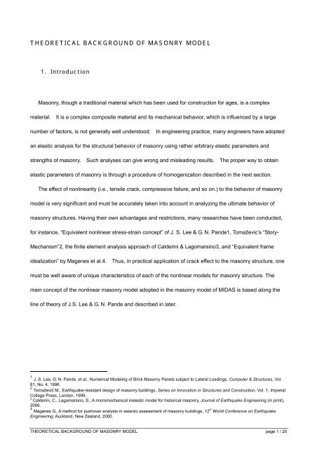
<strong>THEORETICAL</strong> <strong>BACKGROUND</strong> <strong>OF</strong> <strong>MASONRY</strong> <strong>MODEL</strong><br />
1. Introduction<br />
Masonry, though a traditional material which has been used for construction for ages, is a complex<br />
material. It is a complex composite material and its mechanical behavior, which is influenced by a large<br />
number of factors, is not generally well understood. In engineering practice, many engineers have adopted<br />
an elastic analysis for the structural behavior of masonry using rather arbitrary elastic parameters and<br />
strengths of masonry. Such analyses can give wrong and misleading results. The proper way to obtain<br />
elastic parameters of masonry is through a procedure of homogenization described in the next section.<br />
The effect of nonlinearity (i.e., tensile crack, compressive failure, and so on.) to the behavior of masonry<br />
model is very significant and must be accurately taken into account in analyzing the ultimate behavior of<br />
masonry structures. Having their own advantages and restrictions, many researches have been conducted,<br />
for instance, “Equivalent nonlinear stress-strain concept” of J. S. Lee & G. N. Pande1, Tomaževic’s “Story-<br />
Mechanism”2, the finite element analysis approach of Calderini & Lagomarsino3, and “Equivalent frame<br />
idealization” by Magenes et al.4. Thus, in practical application of crack effect to the masonry structure, one<br />
must be well aware of unique characteristics of each of the nonlinear models for masonry structure. The<br />
main concept of the nonlinear masonry model adopted in the masonry model of MIDAS is based along the<br />
line of theory of J.S. Lee & G. N. Pande and described in later.<br />
1 J. S. Lee, G. N. Pande, et al., Numerical Modeling of Brick Masonry Panels subject to Lateral Loadings, Computer & Structures, Vol.<br />
61, No. 4, 1996.<br />
2 Tomaževič M., Earthquake-resistant design of masonry buildings, Series on Innovation in Structures and Construction, Vol. 1, Imperial<br />
College Press, London, 1999.<br />
3<br />
Calderini, C., Lagomarsino, S., A micromechanical inelastic model for historical masonry, Journal of Earthquake Engineering (in print),<br />
2006.<br />
4 Magenes G., A method for pushover analysis in seismic assessment of masonry buildings, 12 th World Conference on Earthquake<br />
Engineering, Auckland, New Zealand, 2000.<br />
<strong>THEORETICAL</strong> <strong>BACKGROUND</strong> <strong>OF</strong> <strong>MASONRY</strong> <strong>MODEL</strong> page 1 / 20
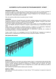
2. Homogenization Techniques in Masonry Structures<br />
Masonry structures can be numerically analyzed if an accurate stress-strain relationship is employed for<br />
each constituent material and each constituent material is then separated individually. However, a threedimension-analysis<br />
of a masonry structure involving even a very simple geometry would require a large<br />
number of elements and the nonlinear analysis of the structure would certainly be intractable. To overcome<br />
this computational difficulty, the orthotropic material properties proposed by Pande et al.5,6 can be<br />
introduced to model the masonry structure in the sense of an equivalent homogenized material. The<br />
equivalent material properties introduced in Pande et al. are based on a strain energy concept. The details<br />
of the procedure to obtain equivalent elastic parameters based on the homogenization technique are given in<br />
the following. The basic assumptions made to derive the equivalent material properties through the strain<br />
energy considerations are:<br />
1. Brick and mortar are perfectly bonded<br />
2. Head or bed mortar joints are assumed to be continuous<br />
The second assumption is necessary in the homogenization procedure and it has been shown7 that the<br />
assumption of continuous head joints instead of staggered joints, as they appear in practice, does not have<br />
any significant effect on the stress states of the constituent materials.<br />
Let the orthotropic material properties of the masonry panel be denoted by<br />
E<br />
x<br />
,<br />
E<br />
y<br />
,<br />
E<br />
z<br />
, ν<br />
xy<br />
, ν<br />
xz<br />
, ν<br />
yz<br />
,<br />
G<br />
xy<br />
,<br />
by<br />
G<br />
yz<br />
,<br />
G<br />
xz<br />
, Fig. 1. The stress/strain relationship of the homogenized masonry material is represented<br />
σ = ⎡ ⎣ D⎤<br />
⎦ ε<br />
(1)<br />
or<br />
5 G. N. Pande, B. Kralj, and J. Middleton. Analysis of the compressive strength of masonry given by the equation<br />
α<br />
( ′) ( )<br />
β<br />
k<br />
=<br />
b m . The Structural Engineer, 71:7-12, 1994.<br />
f K f f<br />
6 G. N. Pande, J. X. Liang, and J. Middleton. Equivalent elastic moduli for brick masonry. Comp. & Geotech., 8:243-265, 1989.<br />
7<br />
R. Luciano and E. Sacco. A damage model for masonry structures. Eur. J. Mech., A/Solids, 17:285-303,1998.<br />
<strong>THEORETICAL</strong> <strong>BACKGROUND</strong> <strong>OF</strong> <strong>MASONRY</strong> <strong>MODEL</strong> page 2 / 20
ε = ⎡ ⎣ C⎤<br />
⎦ σ<br />
(2)<br />
where,<br />
σ =<br />
T<br />
{ σxxσ yyσzzτxyτ yzτxz}<br />
{ xx, yy, zz, xy, yz,<br />
xz}<br />
ε = ε ε ε γ γ γ<br />
T<br />
(3)<br />
are the vectors of stresses and strains in the Cartesian coordinate system.<br />
⎡ 1 ν<br />
xy ν<br />
⎤<br />
xz<br />
⎢ − − 0 0 0 ⎥<br />
⎢<br />
Ex Ex Ex<br />
⎥<br />
⎢ ν<br />
yx 1 ν<br />
⎥<br />
yz<br />
⎢−<br />
− 0 0 0 ⎥<br />
⎢ Ey Ey Ey<br />
⎥<br />
⎢<br />
ν<br />
⎥<br />
⎢ ν<br />
zx zy 1<br />
− −<br />
0 0 0 ⎥<br />
⎢ Ez Ez E<br />
⎥<br />
z<br />
⎡<br />
⎣C⎤ ⎦ = ⎢ ⎥<br />
⎢<br />
1<br />
0 0 0 0 0 ⎥<br />
⎢<br />
G<br />
⎥<br />
xy<br />
⎢<br />
⎥<br />
⎢<br />
1<br />
0 0 0 0 0<br />
⎥<br />
⎢<br />
G ⎥<br />
yz<br />
⎢<br />
⎥<br />
⎢<br />
1 ⎥<br />
⎢ 0 0 0 0 0 ⎥<br />
⎣ Gxz<br />
⎦ (4)<br />
The details of the derivation of orthotropic elastic material properties of masonry in terms of the properties<br />
of the constituents are given in Appendix I. In the mathematical theory of homogenization, there has been<br />
an issue relating to the sequence of homogenization, if there are more than two constituents. For example,<br />
if we homogenize bricks and mortar in head joints first and then homogenize the resulting material with bed<br />
joints at the second stage, then result may not be the same if we had followed a different sequence.<br />
However, it has been shown in the case of masonry, the sequence of homogenization does not have any<br />
significant influence. Here we present in Appendix I equations for equivalent properties if bricks and bed<br />
joints are homogenized first. It is noted that, in Pande et al., the equivalent material properties were derived<br />
with the brick and the head mortar joint being homogenized first. The equivalent orthotropic material<br />
properties derived from the homogenization procedure are used to construct the stiffness matrix in the finite<br />
element analysis procedure and, from this equivalent stress/strains are then calculated. The stresses/strains<br />
in the constituent materials can be evaluated through structural relationships, i.e.,<br />
<strong>THEORETICAL</strong> <strong>BACKGROUND</strong> <strong>OF</strong> <strong>MASONRY</strong> <strong>MODEL</strong> page 3 / 20
σ =<br />
σ<br />
σ<br />
b<br />
[ S ]<br />
b<br />
⎡S<br />
bj<br />
= ⎣ bj ⎦<br />
⎡S<br />
σ<br />
⎤σ<br />
⎤σ<br />
hj<br />
= ⎣ hj ⎦ (5)<br />
where subscripts b, bj and hj represent brick, bed joint ad head joint, respectively.<br />
The structural relationships for strains can similarly be established. The structural matrices S are listed in<br />
Appendix II. From the results listed in Pande et al., it can shown that the orthotropic material properties are<br />
functions of<br />
Fig.1 Coordinate System used in Masonry Panel<br />
1. Dimensions of the brick, length, height and width<br />
2. Young’s modulus and Poisson’s ratio of the brick material<br />
3. Young’s modulus and Poisson’s ratio of the mortar in the head and bed joints<br />
4. Thickness of the head and bed mortar joints<br />
It must be noted that the geometry of masonry has to be modeled in the reference of the above figure. This<br />
is because the homogenization is performed based on the coordinate system.<br />
<strong>THEORETICAL</strong> <strong>BACKGROUND</strong> <strong>OF</strong> <strong>MASONRY</strong> <strong>MODEL</strong> page 4 / 20
3. Criteria for Failure for Constituents<br />
Failure of masonry can be based on the micromechanical behaviour. At every loading step, once the<br />
equivalent stresses/strains in the masonry structure are calculated, stresses/strains of the constituent<br />
materials can be derived based on the structural relationship in eq. (5). The maximum principal stress is<br />
calculated in each constituent level (i.e., Brick, Bed joint, and Head joint) and is compared to the tensile<br />
strength defined by user. If the maximum principal stress exceeds the tensile strength at current step, the<br />
stiffness contribution of the constituent to the whole element is forced to be negligible. For the nonlinear<br />
stress-strain relation of constituents, even the elastio-perfectly plastic relation could be simulated. This can<br />
be numerically implemented by substituting the stiffness of the constituent with very small value as<br />
Ei<br />
zero<br />
(where the subscript ‘i’ could be brick, bed joint, or head joint). If users set the ‘Stiffness Reduction<br />
Factor’ as very small value, the masonry model will behave with nonlinearity. In the same reason, if the<br />
‘Stiffness Reduction Factor’ is set to be unit value, the masonry model will behave elastically (refer to the<br />
figure 2 below).<br />
Fig.2 Stress-Strain of a constituent of masonry model<br />
In this way, the local failure mode can be evaluated. For better understanding this kind of equivalent<br />
nonlinear stress-strain relationship theory, see Lee et al.(1996). Once cracking occurs in any constituent<br />
material, the effect is smeared onto the neighboring equivalent orthotropic material through another<br />
homogenization.<br />
Although there are a number of criteria for the masonry model such as Mohr-Coulomb and so on, the<br />
masonry model in MIDAS currently determines the tensile failure referring only to the user-input tensile<br />
strength. More advanced failure criteria are developed in the near future based on the abundant research.<br />
After the tensile cracks occur, the crack positions can be traced by post processor of solid stresses.<br />
<strong>THEORETICAL</strong> <strong>BACKGROUND</strong> <strong>OF</strong> <strong>MASONRY</strong> <strong>MODEL</strong> page 5 / 20
4. Analysis methods of masonry structures<br />
For the performance assessment of masonry structure, it is generally suggested that the structure needs<br />
to be analyzed in both out-of-plane damage and in-plane damage concepts.<br />
Firstly, referring to the figure 3, the out-of-plane damage which is also called as “first-mode collapse” or<br />
“local damage” involves any kinds of local failure such as tensile failure and partial overturn of masonry wall.<br />
Fig.3 Example of out-of-plane damage mechanism<br />
For the precise analysis of out-of-plane damage of masonry structure, part of the structure is modeled<br />
with detailed finite elements such as material nonlinear models and interface elements to simulate discrete<br />
mortar cracking, interface interaction, shear failure, and etc. This type analysis is numerically expensive and<br />
difficult to simulate real structural response and is not the case in the masonry model of current MIDAS<br />
program.<br />
Secondly, in the reference of figure 4, the in-plane damage which is also called as “second-mode<br />
collapse” means the structural response to the external loading as a whole. MIDAS is providing<br />
homogenized nonlinear masonry model for this kind of analysis. Tensile cracks in mortar and brick can be<br />
traced with simply defined nonlinear masonry material model. It should be noted that the nonlinear behavior<br />
of masonry structure is very sensitive to the material properties such as tensile strength and reduced<br />
stiffness after cracking. So, proper material properties should be carefully defined by thorough investigation<br />
and experimental consideration.<br />
It is widely recognized that the satisfactory behavior of masonry structure is retained only when the outof-plane<br />
damage is well prevented and the structure shows in-plane reaction as a whole. Although these two<br />
types of damage take place simultaneously, the separate detailed analyses are conducted in practical<br />
<strong>THEORETICAL</strong> <strong>BACKGROUND</strong> <strong>OF</strong> <strong>MASONRY</strong> <strong>MODEL</strong> page 6 / 20
easons.<br />
Fig.4 Example of in-plane damage mechanism<br />
<strong>THEORETICAL</strong> <strong>BACKGROUND</strong> <strong>OF</strong> <strong>MASONRY</strong> <strong>MODEL</strong> page 7 / 20
5. Importance of nonlinear analysis of masonry model<br />
To appreciate the importance of nonlinear masonry model, as shown in figure 5, a two story masonry wall<br />
is analyzed linearly and nonlinearly. As suggested by Magenes8, the wall model with openings is subjected<br />
to in-plane simple pushover loadings. The model has 6m-width and 6.5m-height and is meshed by eight<br />
node solid elements.<br />
Firstly the model is analyzed linearly, which means the stiffness reduction factor is set to be unit value, ‘1’.<br />
And then, for nonlinear behavior, the stiffness reduction factor is reduced to have very small value of ‘1.e-10’,<br />
which leads elasto-plastic behavior. The horizontal forces are loaded incrementally with 10 steps, and the<br />
cracked deformed shape at the step 8 is presented in figure 6. The marked points are representing crack<br />
points and the contour results are based on effective stress results.<br />
Fig.5 Two story masonry wall model<br />
8 Guido Magenes, Masonry Building Design in Seismic Areas: Recent Experiences and Prospects from a European Standpoint, First<br />
European Conference on Earthquake Engineering and Seismology, Paper Number: Keynote Address K9, Geneva, Switzerland, 3-8<br />
September, 2006.<br />
<strong>THEORETICAL</strong> <strong>BACKGROUND</strong> <strong>OF</strong> <strong>MASONRY</strong> <strong>MODEL</strong> page 8 / 20
Fig.6 Cracked and deformed shape at step 8<br />
In both cases two models have the same homogenization procedure. The only difference is the reduced<br />
stiffness of a constituent at which the crack took place. The force-displacement result shown in figure 7 gives<br />
that the analytic behavior is significantly dependent on the stiffness of the masonry constituents after crack.<br />
The deformation is extracted from the nodal results of the right top point.<br />
Nonlinear vs. Linear Analysis of Masonry<br />
[ Both cases have the same homogenization ]<br />
9<br />
8<br />
7<br />
Loading Steps<br />
6<br />
5<br />
4<br />
3<br />
2<br />
1<br />
Dx[m]<br />
0<br />
0.0E+00 5.0E-04 1.0E-03 1.5E-03 2.0E-03 2.5E-03 3.0E-03<br />
Nonlinear<br />
Linear<br />
Fig.7 Force-deformation result<br />
<strong>THEORETICAL</strong> <strong>BACKGROUND</strong> <strong>OF</strong> <strong>MASONRY</strong> <strong>MODEL</strong> page 9 / 20
In the reference of figure 8, the significance of nonlinearity is more convincing if we consider the resultant<br />
base shear results. In the figure 8, the horizontal axis is showing the pier positions and the vertical axis is<br />
representing the resultant shear of each pier divided by the total shear force. In the left pier, the base shear<br />
result of nonlinear masonry model is almost half of that of linear masonry model. Contrarily, in the right pier,<br />
the resultant base shear of nonlinear is almost twice that of linear masonry model. Also, overall shear force<br />
distribution is quite different. The linear masonry model shows symmetric force distribution about the mid pier.<br />
In the nonlinear masonry model, however, the right pier has the largest shear force results. From this<br />
consideration, it should be noted that the shear forces after crack are shared not by elastic stiffness but by<br />
the strength capacity as suggested by Magenes(2006).<br />
Nonlinear vs. Linear Analysis of Masonry<br />
[ Both cases have the same homogenization ]<br />
V/Vtotal [%]<br />
55<br />
50<br />
45<br />
40<br />
35<br />
30<br />
25<br />
20<br />
15<br />
10<br />
5<br />
0<br />
Left Pier Mid Pier Right Pier<br />
Nonlinear<br />
Linear<br />
Fig.8 Base shear force distribution<br />
<strong>THEORETICAL</strong> <strong>BACKGROUND</strong> <strong>OF</strong> <strong>MASONRY</strong> <strong>MODEL</strong> page 10 / 20
APPENDIX I<br />
ORTHOTROPIC PROPERTIES <strong>OF</strong> <strong>MASONRY</strong> BASED ON STRAIN ENERGY RULE<br />
Orthotropic material properties of masonry can be derived employing a strain energy concept and the details<br />
are given in the following. It is noted that homogenization is performed between brick and bed joint first.<br />
Similar details can also be obtained when brick and head joint are homogenized first.<br />
Referring to Fig. 1, volume fraction of brick and bed joint can be described as<br />
h<br />
tbj<br />
µ<br />
b<br />
= ; µ<br />
bj<br />
=<br />
h+ t h+<br />
t<br />
bj<br />
bj<br />
A.1<br />
where subscript b and bj represent the brick and bed joint, respectively. If the<br />
brick and bed joint are homogenized in the beginning, the following stress/strain<br />
components in the sense of volume averaging can be established;<br />
{ xx, yy, zz<br />
,<br />
xy, yz,<br />
zx}<br />
T<br />
{ xx, yy, zz, xy, yz,<br />
zx}<br />
σ = σ σ σ τ τ τ<br />
ε = ε ε ε γ γ γ<br />
T<br />
A.2<br />
where,<br />
σ<br />
ε<br />
2<br />
1<br />
= ∑∫ σ dV<br />
A.3<br />
xx xxi i<br />
V<br />
Vi<br />
i=<br />
1<br />
2<br />
1<br />
= ∑∫ ε dV<br />
A.4<br />
xx xxi i<br />
V<br />
Vi<br />
i=<br />
1<br />
and i=1 for brick, i=2 for bed joint. For each strain component,<br />
<strong>THEORETICAL</strong> <strong>BACKGROUND</strong> <strong>OF</strong> <strong>MASONRY</strong> <strong>MODEL</strong> page 11 / 20
1<br />
ε = σ −νσ −νσ<br />
E<br />
( )<br />
xxi xxi i yyi i zzi<br />
i<br />
1<br />
ε = σ −νσ −νσ<br />
E<br />
( )<br />
yyi yyi i xxi i zzi<br />
i<br />
1<br />
ε = σ −νσ −νσ<br />
E<br />
γ<br />
γ<br />
γ<br />
( )<br />
zzi zzi i xxi i yyi<br />
i<br />
xyi<br />
yzi<br />
xzi<br />
τ<br />
=<br />
G<br />
τ<br />
=<br />
G<br />
τ<br />
=<br />
G<br />
xyi<br />
xyi<br />
yzi<br />
yzi<br />
xzi<br />
xzi<br />
A.5<br />
Now the strain energy for each component and 1 layer prism can be denoted as<br />
U<br />
U<br />
2<br />
1<br />
= + + + + +<br />
∑ ∫<br />
( σ ε σ ε σ ε τ γ τ γ τ γ )<br />
re xxi xxi yyi yyi zzi zzi xyi xyi yzi yzi xzi xzi i<br />
1 2<br />
Vi<br />
i=<br />
1<br />
=<br />
2<br />
∫ + + + + +<br />
V<br />
( σ ε σ ε σ ε τ γ τ γ τ γ )<br />
e xx xx yy yy zz zz xy xy yz yz xz xz<br />
dV<br />
dV<br />
A6<br />
where ‘re’ and ‘e’ represent the component and layer prism, respectively, and it is<br />
obvious that<br />
U<br />
re<br />
= U<br />
A7<br />
e<br />
Introduce auxiliary stresses/strains,<br />
σ<br />
σ<br />
σ<br />
τ<br />
τ<br />
τ<br />
xxi xx xxi<br />
yyi<br />
yy<br />
zzi zz zzi<br />
xyi<br />
yzi<br />
= σ + A<br />
= σ<br />
= σ + A<br />
= τ<br />
= τ<br />
xy<br />
yz<br />
= τ + A<br />
xzi xz xzi<br />
A.8<br />
and<br />
<strong>THEORETICAL</strong> <strong>BACKGROUND</strong> <strong>OF</strong> <strong>MASONRY</strong> <strong>MODEL</strong> page 12 / 20
ε<br />
ε<br />
ε<br />
γ<br />
γ<br />
γ<br />
xxi<br />
xx<br />
yyi yy yyi<br />
zzi<br />
zz<br />
xyi xy xyi<br />
yzi yz yzi<br />
xzi<br />
= ε<br />
= ε + B<br />
= ε<br />
= γ + B<br />
= γ + B<br />
= γ<br />
xz<br />
A.9<br />
then, from eqs. (A.3) & (A.8),<br />
2<br />
∑<br />
i=<br />
1<br />
2<br />
∑<br />
i=<br />
1<br />
2<br />
∑<br />
i=<br />
1<br />
µ A<br />
i<br />
µ A<br />
i<br />
µ A<br />
i<br />
xxi<br />
zzi<br />
xzi<br />
= 0<br />
= 0<br />
= 0<br />
A.10<br />
and<br />
2<br />
∑<br />
i=<br />
1<br />
2<br />
∑<br />
i=<br />
1<br />
2<br />
∑<br />
i=<br />
1<br />
µ B<br />
i<br />
µ B<br />
i<br />
µ B<br />
i<br />
yyi<br />
xyi<br />
yzi<br />
= 0<br />
= 0<br />
= 0<br />
A.11<br />
where, µ<br />
1<br />
and µ<br />
2<br />
represent the volume fraction of brick and bed joint, respectively.<br />
From eqs. (A.5),(A.9) & (A.11),<br />
<strong>THEORETICAL</strong> <strong>BACKGROUND</strong> <strong>OF</strong> <strong>MASONRY</strong> <strong>MODEL</strong> page 13 / 20
E<br />
x<br />
2<br />
ζ<br />
= −<br />
α α<br />
1 µ µ<br />
bj ⎛ν b<br />
zy ν ⎞ ⎛ν b<br />
zy<br />
ν ⎞<br />
bj<br />
= + + 2χb⎜ − ⎟+ 2χbj<br />
−<br />
Ey Eb Ebj Ez E ⎜ b<br />
Ez E ⎟<br />
⎝ ⎠ ⎝ bj ⎠<br />
E<br />
z<br />
2<br />
ζ<br />
= α − α<br />
µ<br />
1<br />
G<br />
xy<br />
1<br />
G<br />
G<br />
ν<br />
ν<br />
ν<br />
yz<br />
xz<br />
xy<br />
xz<br />
zy<br />
=<br />
=<br />
=<br />
∑<br />
i<br />
i<br />
∑<br />
i<br />
∑<br />
G<br />
i<br />
xyi<br />
µ<br />
i<br />
G<br />
yzi<br />
( µ G )<br />
χζ<br />
= χ −<br />
α<br />
ζ<br />
=<br />
α<br />
χζ<br />
= χ −<br />
α<br />
xzi<br />
A.12<br />
<strong>THEORETICAL</strong> <strong>BACKGROUND</strong> <strong>OF</strong> <strong>MASONRY</strong> <strong>MODEL</strong> page 14 / 20
where,<br />
µν<br />
b b<br />
χb<br />
=<br />
1 − ν<br />
2 2<br />
( 1− ) + E ( 1−<br />
)<br />
2 2<br />
( 1−νb<br />
)( 1−νbj)<br />
( 1 ) E ( 1<br />
2 2<br />
( 1−νb<br />
)( 1−νbj)<br />
µ<br />
bEb ν<br />
bj<br />
µ<br />
bj bj<br />
νb<br />
α =<br />
µ ν E − ν + µ ν −ν<br />
ζ =<br />
2 2<br />
b b b bj bj bj bj b<br />
b<br />
b<br />
µν<br />
bj bj<br />
χbj<br />
=<br />
1 − ν<br />
bj<br />
χ = χ + χ<br />
bj<br />
)<br />
A.13<br />
and the relationship below can also be established;<br />
ν<br />
yx<br />
E<br />
y<br />
= ν<br />
xy<br />
A.14<br />
Ex<br />
For the system of masonry panel, the homogenization is applied to the layered material and head joint based<br />
on the assumption of continuous head joint. Now, volume fractions of the constituent materials are<br />
l<br />
thj<br />
µ<br />
eq<br />
= ; µ<br />
hj<br />
= A.15<br />
l + t l + t<br />
hj<br />
hj<br />
where, subscript eq and hj represent layered material and head joint, respectively. As in the previous case,<br />
the following stress/strain components in the sense of volume averaging can be established;<br />
{ xx, yy, zz, xy, yz,<br />
zx}<br />
T<br />
{ xx, yy, zz<br />
,<br />
xy, yz<br />
,<br />
zx}<br />
σ = σ σ σ τ τ τ<br />
ε = ε ε ε γ γ γ<br />
T<br />
A.16<br />
<strong>THEORETICAL</strong> <strong>BACKGROUND</strong> <strong>OF</strong> <strong>MASONRY</strong> <strong>MODEL</strong> page 15 / 20
Introducing auxiliary stresses/strains,<br />
σ<br />
σ<br />
σ<br />
τ<br />
τ<br />
τ<br />
xxi<br />
xx<br />
yyi yy yyi<br />
zzi zz zzi<br />
xyi<br />
xy<br />
yzi yz yzi<br />
xzi<br />
= σ<br />
= σ + C<br />
= σ + C<br />
= τ<br />
= τ + C<br />
= τ<br />
xz<br />
A.17<br />
and<br />
ε<br />
ε<br />
ε<br />
γ<br />
γ<br />
γ<br />
xxi xx xxi<br />
yyi<br />
zzi<br />
yy<br />
zz<br />
xyi xy xyi<br />
yzi<br />
= ε + D<br />
= ε<br />
= ε<br />
= γ + D<br />
= γ<br />
yz<br />
= γ + D<br />
xzi xz xzi<br />
A.18<br />
where, i=1 & i=2 represent the layered material and head joint, respectively. Following the same procedure<br />
and defining the following coefficients,<br />
µ E µ E<br />
α = +<br />
1−ν ν 1<br />
eq y hj hj<br />
2<br />
yz zy<br />
−νhj<br />
µ E µ E<br />
β = +<br />
1−ν ν 1<br />
eq z hj hj<br />
2<br />
yz zy<br />
−νhj<br />
µν E µν E<br />
ζ = +<br />
1 1<br />
eq yz z hj hj hj<br />
2<br />
−ν yzνzy −νhj<br />
eq<br />
( + )<br />
µ<br />
eq<br />
νzx ν<br />
yxνzy<br />
χeq<br />
=<br />
1−ν ν<br />
µν<br />
hj hj<br />
χhj<br />
=<br />
1 − ν<br />
hj<br />
χ = χ + χ<br />
hj<br />
yz<br />
zy<br />
<strong>THEORETICAL</strong> <strong>BACKGROUND</strong> <strong>OF</strong> <strong>MASONRY</strong> <strong>MODEL</strong> page 16 / 20
eq<br />
( + )<br />
µ<br />
eq<br />
ν<br />
yx<br />
ν<br />
yzνzx<br />
λeq<br />
=<br />
1−ν ν<br />
µν<br />
hj hj<br />
λhj<br />
=<br />
1 − ν<br />
hj<br />
λ = λ + λ<br />
hj<br />
yz<br />
zy<br />
A.19<br />
the orthotropic material properties of the masonry panel are finally derived;<br />
1 µ<br />
eq<br />
µ ⎛<br />
hj<br />
ν<br />
yx<br />
ν ⎞ ⎛<br />
xy<br />
ν<br />
yx<br />
ν ⎞<br />
hj<br />
= + + λeq<br />
− + λhj<br />
−<br />
Ex Ex E ⎜ hj<br />
Ey E ⎟ ⎜<br />
+<br />
⎝ x ⎠ ⎝ Ey E ⎟<br />
hj ⎠<br />
E<br />
y<br />
2<br />
αβ −ζ<br />
Ez<br />
=<br />
α<br />
1 µ<br />
eq<br />
µ<br />
hj<br />
= +<br />
G G G<br />
1 µ<br />
eq<br />
µ<br />
hj<br />
= +<br />
G G G<br />
2<br />
xy xy hj<br />
G = µ G + µ G<br />
ν<br />
ν<br />
ν<br />
ν<br />
yz eq yz hj hj<br />
xz xz hj<br />
yx<br />
yz<br />
zx<br />
zy<br />
⎛νzx ν ⎞ ⎛<br />
xz<br />
ν ν ⎞<br />
zx hj<br />
χeq<br />
⎜ − ⎟+ χhj<br />
−<br />
Ez E ⎜ x<br />
Ez E ⎟<br />
⎝ ⎠ ⎝ hj ⎠<br />
αβ −ζ<br />
=<br />
β<br />
ζχ<br />
= λ −<br />
β<br />
=<br />
ζ<br />
β<br />
ζλ<br />
= χ −<br />
α<br />
ζ<br />
=<br />
α<br />
A.20<br />
<strong>THEORETICAL</strong> <strong>BACKGROUND</strong> <strong>OF</strong> <strong>MASONRY</strong> <strong>MODEL</strong> page 17 / 20
APPENDIX II<br />
STRUCTURAL RELATIONSHIP <strong>OF</strong> <strong>MASONRY</strong><br />
Structural relationship of each constituent materials with respect to overall masonry can be established<br />
through utilizing auxiliary stress/strain components introduced in Appendix I. Details of each relationship are<br />
now deduced.<br />
As in eq. (5), the structural matrix has the following form;<br />
[ S]<br />
⎡S S S<br />
⎢<br />
⎢<br />
S S S<br />
⎢S S S<br />
11 12 13<br />
21 22 23<br />
31 32 33<br />
= ⎢<br />
⎢ 0 0 0 S44<br />
0 0 ⎥<br />
⎢ 0 0 0 0 S55<br />
0 ⎥<br />
⎢<br />
⎥<br />
⎢⎣<br />
0 0 0 0 0 S66<br />
⎥⎦<br />
0 0 0 ⎤<br />
0 0 0<br />
⎥<br />
⎥<br />
0 0 0 ⎥<br />
⎥ A.21<br />
Solving the auxiliary stress/strain components in eqs. (A.17) & (A.18),<br />
σ<br />
= σ + C<br />
yy, hj yy yy,<br />
hj<br />
2<br />
{ Ehjεyy νhjEhjεzz ( νhj νhj ) σxx}<br />
1<br />
= + + +<br />
1−νν<br />
hj<br />
hj<br />
⎧⎪ ν ⎛ν νν ⎞⎫⎪ ⎧⎪ ⎛ 1 νν ⎞⎫⎪ ⎧⎪<br />
⎛ν ν<br />
= σxx ⎨ − η + + σ<br />
yy<br />
η − + σzz<br />
η −<br />
1 ν ⎜ E E ⎟⎬ ⎨ ⎜ ⎬ ⎨<br />
E E ⎟ ⎜<br />
⎪⎩ − ⎝ ⎠⎪⎭ ⎪⎩ ⎝ ⎠⎪⎭ ⎪⎩<br />
⎝ E E<br />
hj yx hj zx hj zy hj yz<br />
hj y z y z z y<br />
⎞⎫<br />
⎪<br />
⎟⎬ ⎟ ⎠⎪<br />
⎭<br />
A.22<br />
where,<br />
E<br />
η = A.23<br />
1 − ν<br />
hj<br />
2<br />
hj<br />
Therefore,<br />
<strong>THEORETICAL</strong> <strong>BACKGROUND</strong> <strong>OF</strong> <strong>MASONRY</strong> <strong>MODEL</strong> page 18 / 20
S<br />
S<br />
S<br />
hj xy hj zx<br />
hj,21 2<br />
1 ν ⎜<br />
hj<br />
Ey Ez<br />
hj,22<br />
hj,23<br />
ν ⎛ν ν ν ⎞<br />
= − η +<br />
− ⎟<br />
⎝ ⎠<br />
⎛ 1 νν ⎞<br />
hj zy<br />
= η<br />
−<br />
⎜<br />
Ey<br />
E ⎟<br />
⎝<br />
z ⎠<br />
⎛νhj<br />
ν<br />
= η<br />
−<br />
⎜<br />
⎝ Ez<br />
E<br />
yz<br />
y<br />
⎞<br />
⎟<br />
⎠<br />
A.24<br />
The above equation can be rewritten as follows:<br />
S<br />
S<br />
S<br />
hj,21<br />
hj,22<br />
hj,23<br />
ν ⎛<br />
hj<br />
ν<br />
yx<br />
νhjν<br />
⎞<br />
zx<br />
= − ηhj<br />
+<br />
1−ν<br />
⎜<br />
hj<br />
Ey E ⎟<br />
⎝ z ⎠<br />
⎛ 1 νν ⎞<br />
hj zy<br />
= ηhj<br />
−<br />
⎜<br />
Ey<br />
E ⎟<br />
⎝<br />
z ⎠<br />
⎛νhj<br />
ν<br />
= ηhj<br />
−<br />
⎜<br />
⎝ Ez<br />
E<br />
yz<br />
y<br />
⎞<br />
⎟<br />
⎠<br />
A.25<br />
where,<br />
η<br />
hj<br />
E<br />
= A.26<br />
1 − ν<br />
hj<br />
2<br />
hj<br />
Using same procedure, the remaining non-zero coefficients can also be derived;<br />
S<br />
S<br />
S<br />
S<br />
S<br />
S<br />
S<br />
hj,11<br />
hj,31<br />
hj,32<br />
hj,33<br />
hj,44<br />
hj,55<br />
hj,66<br />
= 1.0<br />
ν ⎧<br />
hj ⎪νhjν yx ν ⎫<br />
zx ⎪<br />
= − ηhj<br />
⎨ + ⎬<br />
1−ν<br />
hj ⎪⎩<br />
Ey Ez<br />
⎪⎭<br />
⎧⎪ν<br />
hj ν ⎫<br />
zx ⎪<br />
= ηhj<br />
⎨ − ⎬<br />
⎪⎩Ey<br />
Ez<br />
⎪⎭<br />
⎧⎪<br />
1 νν ⎫<br />
hj yz ⎪<br />
= ηhj<br />
⎨ − ⎬<br />
⎪⎩Ez<br />
Ey<br />
⎪⎭<br />
= 1.0<br />
G<br />
=<br />
G<br />
hj<br />
yz<br />
= 1.0<br />
A.27<br />
<strong>THEORETICAL</strong> <strong>BACKGROUND</strong> <strong>OF</strong> <strong>MASONRY</strong> <strong>MODEL</strong> page 19 / 20
Solving for the unknowns A, B, C and D in eqs. (A.8), (A.9), (A.17) and (A.18), the structural matrix for each<br />
component can be derived and the full details will be omitted.<br />
<strong>THEORETICAL</strong> <strong>BACKGROUND</strong> <strong>OF</strong> <strong>MASONRY</strong> <strong>MODEL</strong> page 20 / 20