The Composite Radiosity and Gap (CRG) Model of Thermal Radiation

The Composite Radiosity and Gap (CRG) model of Thermal Radiation
ABSTRACT
Niels Bjarne K. Rasmussen
Danish Gas Technology Centre a/s
DK-2970 Hørsholm, Denmark
nbr@dgc.dk
INFUB 2002 Conference, Estoril – Lisbon - Portugal
Calculating the thermal radiation in furnaces and boilers has always been a problem of
choosing between complexity and simplicity which are related to high and low calculation
time. The best choice will always be somewhere in between using models that are complex
enough to describe the problem adequately and at the same time simple enough to be understood
and used by the user.
Especially in CFD you have to choose an economical model to get a solution within reasonable
computing time. This new CRG-model of thermal radiation fits in that point. It gives
analytically correct results for a number of examples covering the range between optically
thick and optically thin cases and cases without participating medium (wall to wall radiation).
The equation solved in the CRG-model is a simple diffusion equation. However, the model
should not be mistaken for being the Diffusion model of radiation, which only works for optically
very thick cases. For optically thick cases the CRG-model gives the same correct solution
as the Diffusion method, while for optically thin cases (thickness zero) it gives the same
solution as a simple wall to wall calculation. For two opposing infinite walls it gives the analytical
solution. For any other geometry it gives plausible results.
The bases of the CRG model are two models of Spalding: The Radiosity model and the IM-
MERSOL model. The Radiosity model gives good results for optically thick cases like the
Diffusion model, but it has a wider span than the diffusion model, meaning that it goes to a
lower optical thickness. The IMMERSOL model by Spalding is made for calculating the radiation
between IMMERsed SOLids in the topical fluid. The CRG model and the IMMER-
SOL model have a lot in common, but CRG is more rigorously deduced than shown at the
CHAM home page about IMMERSOL.
The CRG model can be expanded to use “Band models” and “Sum of Grey Gases” and that
without expanding the calculation time considerably. Some errors are corrected in the CRG
model compared to the IMMERSOL.
The basic idea of the CRG model is to define a kind of “geometrical determined resistance of
radiation” for any point in the geometry. This additional “resistance” is based on a local figure
of the “Gap” between the walls at that particular location. The calculation of the local “Gap”
is done by a method also found by Spalding.
The CRG model has been implemented as a user-subroutine in the CFD code STAR-CD. It
gives excellent results and by a minimum of calculation time.
Examples of the use of the CRG model for furnace calculations and for use in optimising radiant
burners are presented.
Keywords: Thermal radiation model, Composite Radiosity Gap (CRG), CFD, isotropic
absorption, scattering, band model, grey gases.

Introduction
In most cases radiation models are used for finding the radiant source and sink terms for CFD
modelling. These terms are then put into the transport equation for enthalpy giving the temperature
distribution in the topical case. Other results from the radiation models are the heat
fluxes and heat transfer to the walls of the case in question. From this information the heat
load on the boiler tubes or the furnaces walls can be calculated.
Many models for thermal radiation include constants for the absorption coefficient a and
for the mean beam length L m . This is adequate for some special cases as cubic or spherical
geometries with almost constant temperatures and concentrations. However, in most cases it
is necessary to be able to use varying values of the mean beam length and the absorption. In
the CRG-model there are no restrictions for the variation of these variables. However, the
absorption and the scattering must be isotropic.
The sink term of any point in the furnace is rather easily calculated, given from the fact that
this term is only dependent on the conditions of the point in question. The source term at any
point related to thermal radiation is however dependent on the condition of the whole furnace
or geometry in question. The present model focuses on calculation of the source term for the
thermal radiation.
The Radiosity model
The flux equation of thermal radiation, which is valid regardless of the optical thickness /1/, is
given by:
dqi
= 4 a( eb
− R)
[W/m 3 ] (1)
dx
i
where q i is the radiant flux. The term e b is given by :
4
e b
= σT
[W/m 2 ] (2)
Above a is the absorption coefficient, σ is the Stefan Boltzmanns constant and T is
the temperature in Kelvin of the fluid. The term R is the radiosity (W/m 2 ) which is the
incoming radiation at any point. The total source term for the energy equation /1/ is found by:
S
rad
dq
( R − e )
i
= − = 4 a
b
[W/m 3 ] (3)
dxi
As pointed out above the sink term is relatively easily calculated. It is given by the equation:
S
rad, sink
4
= −4aσT
[W/m 3 ] (4)
The source term of radiation is much more difficult to calculate. The source term is found as
the radiation coming in from all directions towards the topical point. This term is dependent
on the conditions in all parts of the geometry, as thermal radiation does not follow the standard
transport equation for a fluid scalar, and it comes from walls as well as from the gas itself.

For optically thick cases this term can be found by the Radiosity equation /1, 2/. The Radiosity
equation is found by setting up the approximation:
q
i
4 dR
= −
[W/m 2 ] (5)
3k
dx
i
which combined with equation (1) gives the Radiosity equation:
d ⎛ 4 dR ⎞
0 = a( eb
− R)
dx
⎜
i
k dx
⎟ + 4
[W/m 3 ] (6)
⎝ 3
i ⎠
The extinction coefficient k is given by:
k = a + s
[m -1 ] (7)
where s is the scattering coefficient.
The Radiosity equation is valid for optically thick cases. However, it fails for optically thin to
medium cases, which are the most common. The next section shows how to overcome this
problem.
The Composite Radiosity and Gap (CRG) model
For optically very thick cases the fluid almost “can’t see” the walls around the fluid because
of the optical thickness. However, for optically thin cases the walls are of importance. One
case in which the analytical solution is known is the radiation between infinite plates of different
temperature. The fluid in between is not participating in the radiation, i.e. the absorption
and scattering are zero. The walls are black. The radiant flux between such plates is
found by:
q
= −∆
[W/m 2 ] (8)
y
e b
in which the direction y is a normal to the plates. The term ∆e b is equal to σ(T 2 4 -T 1 4 ) .
It is now assumed that a solution for R between the plates can be found by the approximation:
∆e b dR
=
D dy
[W/m 3 ] (9)
The term D is the gap (distance) between the two walls. Equations 8 and 9 can be combined
to give:
dR
q y
= −D
[W/m 2 ] (10)
dy

By comparing the equations (10) and (5) it is obvious that there is a kind of analogy between
the “stopping distance” 1/k related to the absorption of the fluid in the optically thick case
and the effective geometrical “stopping distance” D in the optically thin case /2/. Now,
taking the term k as being the “resistance of radiation” in the optically thick case and 1/D
as being the “geometrical resistance” in the optically thin case, these two resistances can be
summed up to give the resulting total extinction for calculation of the Radiosity R :
4
k' = k +
[m -1 ] (11)
3D
The weight between k and 1/D could be different from the above but calculations of
different cases show that equation (11) gives good results. The resulting equation of the CRGmodel
is then given by:
d ⎛ 4 dR ⎞
0 = + ( aT
eb
− aRR)
dx
⎜
i
k dx
⎟ 4
[W/m 3 ] (12)
⎝ 3 '
i ⎠
In this equation the terms k’ and a may be constants. However, for most cases they are
not constants and equation (12) can be solved for varying values of these terms. If gas radiation
is considered the terms a T and a R may be different. This is due to the fact that the
absorption a of gasses is temperature dependent. The temperature related to the Radiosity
R is found by:
( R /σ ) 1/ 4
T R
= [K] (13)
The absorptions a T and a R are then found at the temperatures T gas and T R .
Equation (12) is merely a diffusion equation and is analogous to the conduction equation in
solids including an energy source term.
Now, let us look at equation (12) for different cases. When we have the optically thin case
with radiation between two infinite plates the equation (12) reduces to:
d ⎛ dR ⎞
0 =
⎜ D
⎟
[W/m 3 ] (14)
dxi ⎝ dx i ⎠
4
When adding the boundary conditions at solid walls R w = σT w and solving for R the
solution is found to satisfy the equation (8) for this case. In other words, equation (12) gives
the analytically correct solution for this case.
In the optically thick case the equation (12) reduces to equation (6), the Radiosity equation.
As pointed out this equation is valid for optically thick cases. The question is now, how does
the equation (12) behave in the case of medium optical thickness and how about the boundary
conditions (BC). This is shown in the next section.

Boundary conditions
The obvious boundary condition (BC) at walls is to extend the BC at the optically thin case to
all cases (R w = σT w 4 ). However, this gives wrong solutions for optically medium and thick
cases with energy source terms. In references /3/ and /4/ some analytical solutions for cases
with medium optical thickness can be found. The cases have infinite parallel walls as above,
but the walls have the temperature of 0K, the fluid participates with optical thickness from 0.1
to 2.0, and a constant energy source term is introduced in the fluid. Only radiant heat transfer
is considered. There is a wall slip in temperature. This case could be considered as an idealised
boiler situation with radiation from the fluid to the boiler walls and energy release by
combustion in the fluid.
Using equations (11) and (12) on this case gives solutions of the temperature within 2% of the
correct analytical solutions. However, special BC’s have to be introduced for R . Using the
BC’s from above gives too small temperatures and too small radiosities. The following BC
gives the correct solution:
R
w
4
w
σT
+ C
=
1+
C
aD
aD
σT
4
c
[W/m 2 ] (15)
in which
C aD
= ln( aD +1) / ln(2)
(16)
In equation (15) T c is the temperature of the participating fluid in the computational cell
adjacent to the topical wall boundary cell, or even better, the extrapolated fluid temperature at
the wall (wall slip). The equations (15) and (16) are empirical equations. It might be possible
to find even better equations but the above give very good results. The meaning of equation
(15) is to change the BC at the wall in relation to the optical thickness aD of the case. With
4
no participating fluid the BC for R is σT w . With a participating fluid the BC for R
4
gets closer to σT c dependent on the optical thickness.
When the emissivity of the walls are less than 1.0 some additional resistance of R at the
walls must be introduced. From analytical solutions of the case with infinite walls above it
can be deduced that the following transfer coefficient should be used at walls:
h
R
⎛ 3⋅∆y
⋅k'
1
=
⎜ +
⎝ 4 ε
w
⎞
−1
⎟
⎠
−1
[-] (17)
The terms ∆y and ε w are the distance from the wall to the cell mid point and the wall
emissivity, respectively. Equation (17) gives the transfer coefficient for R between the cell
adjacent to the wall and the wall. The flux of R at walls is equal to the total radiant flux at
the walls.
Special boundary conditions are necessary at baffles with heat conduction and for conjugate
heat transfer.

Calculation of the Gap
In the cases presented above the gap D between the walls is very easily found. It is merely
the distance between the plates. However, in general the gap is not that easily found. In such
cases the gap is found by a method described in /2/. A variable L is defined. The equation
for L is:
d ⎛ dL ⎞
0 =
⎜
⎟ +1
(18)
dxi ⎝ dx i ⎠
This is another diffusion equation. L has the unit of (m 2 ) but it has no physical meaning.
The BC of L is zero at all walls. From L it is possible to deduce the gap at any point in
the geometry.
2
⎡⎛
dL ⎞ ⎤
D = 2⎢
⎜
⎟ + 2L⎥
⎢⎣
⎝ dxi
⎠ ⎥⎦
0.5
[m] (19)
Using equations (18) and (19) the gap related to any point in the geometry can be found. In
the case of infinite plates above the solution will be the distance between the plates. In any
other case the solution will be a very plausible measure of the gap at that point. The gap D
is not a constant in an arbitrary shaped case. It will vary through the geometry.
Band models and sum of grey gases
The model is easily expanded to calculation of band models or sum of grey gases for radiation.
The Radiosity equation is solved for each band or gas j and gives different R j for
each band. The absorption a j and the scattering s j of each band or gas is used and proper
BC’s included. The total radiant source is then:
( a R a e )
S = ∑4 −
[W/m 3 ] (20)
rad
j
Rj
j
Tj
b
When calculating the absorption coefficient of the participating gas a g the mean beam
length L m of the radiation in the geometry has to be found. In most cases the a g is dependent
on L m , which is a geometrical term only dependent on the local geometry. For infinite
parallel plates in the examples above the L m is found by:
L m
= 2D
[m] (21)
This equation is assumed to be valid for all geometries. Traditionally, in many radiation models
L m were assumed to be a constant throughout the geometry. With the above assumptions
L m may vary which is very plausible and logical. L m given by (21) is only the geometrical
mean beam length. In cases where absorbing fluids are present, the effective mean
beam length is reduced accordingly, and it is calculated by a method not presented here.

Examples of the use of the CRG radiation model
As shown above in the two analytical described cases with infinite walls the CRG model
gives exact results within a few percent. Theoretically, for optically thick cases the CRG
model gives exact results as the diffusion model. Some other examples of the use of this
model will be given below.
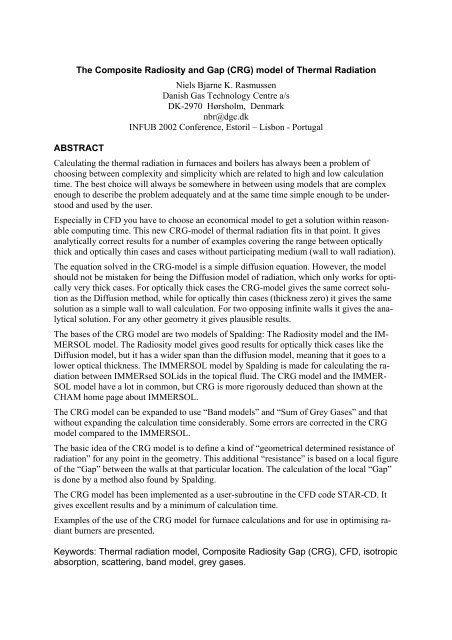
a) Flow and radiation in a confined self-recuperative radiant burner
To be able to predict the conditions inside a confined self-recuperative burner the CRG model
has been used to calculate the radiant heat transfer inside. The heat exchange is partly by convection
and partly by thermal radiation. The flow and radiation was calculated by the use of
the STAR-CD CFD-model and including the CRG model in user-subroutines. With the calculations
it was possible to predict possible performance for improved prototypes of the
burner compared to the original. Below in Figure 1 and 2 is an example of calculation of the
temperature field and the radiosity field for this burner.
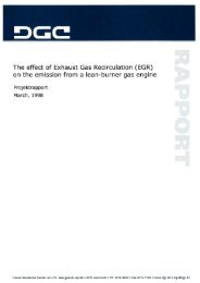
b) Flow and heat transfer in a burner tube for liquid heating
The CRG-model has been used in CFD calculations of a burner tube for heating of liquids.
The purpose was to find the maximum tube temperature at any point to see the risk of boiling
on the outside and to compare with information from the manufacturer of the burner tube. The
results turned out to be very close to the information from the manufacturer, which was based
on measurements. In the Figures 3 and 4 below the calculated temperature and radiosity in a
plane through the axis of the tube are shown.
c) Flow, combustion and radiation in a glass furnace with flame less oxidation
In the third case the CRG model has been combined with an advanced combustion model for
natural gas combustion in a glass furnace with a flame less oxidation burner. The combustion
has been modelled including about 200 chemical reactions and 50 species. In this model the
EDK model for combining turbulence and combustion has been used. The EDK model was
presented at the INFUB97 conference. The CRG model has been included for the thermal
heat transfer. The absorption coefficient of the gases is varying in the geometry dependent of
the concentrations, the temperature and the mean beam length of radiation.
Conclusions
A new model for thermal radiation has been developed. The model is called the Composite
Radiosity and Gap (CRG) model. The model is very economical in use, as the equations to be
solved are pure diffusion equations. The model should not be mistaken for being the Diffusion
model of radiation, which only works for optically very thick cases. The CRG model
covers the whole range from optically very thin cases to optically thick cases. As shown
above in the two analytically described cases with infinite walls the CRG model gives exact
results within a few percent. This is totally adequate for practical use of the model in CFD and
in pure radiation cases. The model gives very plausible results in cases where the exact result
is not known.
The model is very easily implemented in CFD models for combustion and fluid flow. The
absorption and scattering coefficients, the mean beam length for radiation and the calculated
“gap” at any point may vary throughout the geometry and need not be constants. The absorption
and scattering must be isotropic.
Special boundary conditions have to be included for walls and baffles and in case of conjugate
heat transfer.

STAR
PROSTAR 3.10
13-Sep-01
TEMPERATURE
RELATIVE
CELSIUS
ITER = 6957
LOCAL MX= 771.7
LOCAL MN= 37.00
750.0
700.0
650.0
600.0
550.0
500.0
450.0
400.0
350.0
300.0
250.0
200.0
150.0
100.0
50.00
Z
Y
X
Figure 1. The calculated temperature field inside of the confined burner. (°C)
STAR
PROSTAR 3.10
28-Nov-01
SC 2-R
ITER = 6957
LOCAL MX= 0.4887E+05
LOCAL MN= 573.9
0.4200E+05
0.3900E+05
0.3600E+05
0.3300E+05
0.3000E+05
0.2700E+05
0.2400E+05
0.2100E+05
0.1800E+05
0.1500E+05
0.1200E+05
9000.
6000.
3000.
-0.3906E-02
Z
Y
X
Figure 2. The calculated radiosity field inside of the confined burner. (W/m 2 )

STAR
PROSTAR 3.10
28-Nov-01
TEMPERATURE
ABSOLUTE
KELVIN
ITER = 957
LOCAL MX= 1820.
LOCAL MN= 298.5
1834.
1703.
1572.
1441.
1310.
1179.
1048.
917.0
786.0
655.0
524.0
393.0
262.0
131.0
0.0000E+00
Y
X
Z
Figure 3. The calculated temperature in a plane through the axis of the tube. (K)
STAR
PROSTAR 3.10
28-Nov-01
SC 2-R
ITER = 957
LOCAL MX= 0.4788E+05
LOCAL MN= 1070.
0.5001E+05
0.4644E+05
0.4286E+05
0.3929E+05
0.3572E+05
0.3215E+05
0.2858E+05
0.2500E+05
0.2143E+05
0.1786E+05
0.1429E+05
0.1072E+05
7144.
3572.
-0.3906E-02
Y
X
Z
Figure 4. The calculated radiosity in a plane through the axis of the tube. (W/m 2 )

STAR
PROSTAR 3.10
05-Mar-01
TEMPERATURE
ABSOLUTE
KELVIN
ITER = 681
LOCAL MX= 1778.
LOCAL MN= 1402.
1750.
1675.
1600.
1525.
1450.
1375.
1300.
1225.
1150.
1075.
1000.
925.0
850.0
775.0
700.0
Y
FLOX optimization
X
Z
Figure 5. The calculated temperature field in a glass furnace. (K)
STAR
PROSTAR 3.10
05-Mar-01
SC 2-R
ITER = 681
LOCAL MX= 0.2762E+06
LOCAL MN= 7334.
0.2700E+06
0.2600E+06
0.2500E+06
0.2400E+06
0.2300E+06
0.2200E+06
0.2100E+06
0.2000E+06
0.1900E+06
0.1800E+06
0.1700E+06
0.1600E+06
0.1500E+06
0.1400E+06
0.1300E+06
Y
FLOX optimization
X
Z
Figure 6. The calculated radiosity field in a glass furnace. (W/m 2 )

STAR
PROSTAR 3.10
05-Mar-01
SC 5-ABC(IC)
ITER = 681
LOCAL MX= 3.189
LOCAL MN= 0.4623E-02
0.7000
0.6500
0.6000
0.5500
0.5000
0.4500
0.4000
0.3500
0.3000
0.2500
0.2000
0.1500
0.1000
0.5000E-01
0.0000E+00
Y
FLOX optimization
X
Z
Figure 7. The calculated absorption coefficient in a glass furnace. (m -1 )
References
/1/ R. Siegel and J. R. Howell, Thermal Radiation Heat Transfer , Hemisphere, 1992
/2/ Brian Spalding, Radiative Heat Transfer in Phoenics, CHAM home page,
http://www.cham.co.uk/, 2001
/3/ M. A. Heaslet and R. F. Warming, Radiative transport and wall temperature slip in an absorbing
planar medium, Int. J. Heat Mass Transfer 8, 979-994, 1965
/4/ N. B. K. Rasmussen et al., Numerical Integration Method of Radiative Exchange (NIM-
REX), Int. J. Heat Mass Transfer 32, 343-350, 1989