A Neuro-Fuzzy Approach to Hybrid Intelligent Control - ResearchGate
A Neuro-Fuzzy Approach to Hybrid Intelligent Control - ResearchGate
A Neuro-Fuzzy Approach to Hybrid Intelligent Control - ResearchGate

Create successful ePaper yourself
Turn your PDF publications into a flip-book with our unique Google optimized e-Paper software.
A <strong>Neuro</strong>-<strong>Fuzzy</strong> <strong>Approach</strong> <strong>to</strong> <strong>Hybrid</strong> <strong>Intelligent</strong><br />
<strong>Control</strong><br />
B. Lazzerini, L.M. Reyneri, M. Chiaberge<br />
Abstract<br />
This paper presents a neuro-fuzzy approach <strong>to</strong> the development<br />
of high-performance real-time intelligent and adaptive<br />
controllers for non-linear plants. Several paradigms derived<br />
from cognitive sciences are considered and analyzed<br />
in this work, such as Neural Networks, <strong>Fuzzy</strong> Inference<br />
Systems, Genetic Algorithms, etc. The dierent control<br />
strategies are also integrated with Finite State Au<strong>to</strong>mata,<br />
and the theory of <strong>Fuzzy</strong> State Au<strong>to</strong>mata is derived from<br />
that. The novelty of the proposed approach resides in the<br />
tight integration of the control strategies and in the capability<br />
of allowing a hybrid design. Finally, three practical<br />
applications of the proposed hybrid approach are analyzed.<br />
I. Introduction<br />
During the last years several methodologies have shown<br />
up in the eld of \intelligent control" [1], like fuzzy [2],<br />
neural [3] and genetic control [4], providing for the rst<br />
time practical solutions for non-linear control problems, or<br />
supplying better or at least alternative solutions for some<br />
classical problems. Each ofthese new approaches has its<br />
own advantages and drawbacks, and that explains why they<br />
have been applied only <strong>to</strong> specic elds.<br />
As no solution seems appropriate <strong>to</strong> solve by itself most<br />
problems, we developed and tested a hybrid approach that<br />
merges one or more of the following control paradigms:<br />
fuzzy control, neural control, linear control, optimization<br />
algorithms like simulated annealing and genetic optimization,<br />
and nite state au<strong>to</strong>mata [5], and nally the new theory<br />
of <strong>Fuzzy</strong> State Au<strong>to</strong>mata [6], [7].<br />
An immediate synergy can be found between fuzzy and<br />
neural control. The former exploits an important feature<br />
of <strong>Fuzzy</strong> Systems (FSs), that is the capability <strong>to</strong><br />
build the rule base by acquiring the knowledge from human<br />
experts (human-friendly approach). On the other<br />
hand, Neural Networks (NNs) are trained with a suitable<br />
set of data samples (computer-friendly approach), without<br />
though taking advantage from available human knowledge.<br />
Recently, NNs and FSs have been unied [6] using the<br />
Weighted Radial Basis Functions (WRBFs) paradigm [8],<br />
by means of which fuzzy rules and neurons can immediately<br />
be mapped on<strong>to</strong> each other, and then trained or optimized<br />
in the same way as traditional NNs, using gradient descent<br />
methods. This can lead <strong>to</strong> a noticeable increase in performance<br />
and ease of development, since it allows <strong>to</strong> optimize<br />
with gradient descent methods a network previously initialized<br />
with an approximate solution provided by the human<br />
expert as a set of fuzzy rules. This often avoids the local<br />
minima problem typical of NNs.<br />
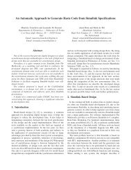
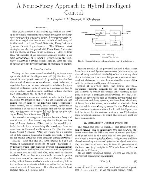
Fig. 1.<br />
Setpoints<br />
<strong>Control</strong>ler<br />
Optimizer<br />
Main <strong>Control</strong> loop<br />
Plant<br />
Error<br />
Evalua<strong>to</strong>r<br />
Learning/Adapting loop<br />
Outputs<br />
General structure of an adaptive control architecture.<br />
Another novelty ofthe proposed method is that, apart<br />
from the static and dynamic parameters (which may be optimized<br />
using traditional methods), other interesting plant<br />
characteristics, suchaspower dissipation, componentwear,<br />
mechanical stresses, etc, may be optimized by means of Genetic<br />
Algorithms and Simulated Annealing.<br />
Section II describes briey the neural and fuzzy<br />
paradigms currently available for the design of intelligent<br />
controllers; section III compares these paradigms and<br />
points out their advantages and drawbacks. Section IV describes<br />
the problems arising in recurrent models using neural<br />
networks and fuzzy systems, and introduces the theory<br />
of <strong>Fuzzy</strong> State Au<strong>to</strong>mata, as a method <strong>to</strong> deal with feedback<br />
inhybrid neuro-fuzzy systems. Section V describes a<br />
few hardware implementations for hybrid intelligent control<br />
developed by the authors, while section VI describes<br />
three practical examples, <strong>to</strong> which the proposed methods<br />
have been applied.<br />
II. <strong>Intelligent</strong> <strong>Control</strong> Paradigms<br />
The paradigms used <strong>to</strong> design <strong>Hybrid</strong> <strong>Intelligent</strong> <strong>Control</strong>lers<br />
(HICs) can be divided in<strong>to</strong> two groups: NNs, FSs,<br />
linear controllers like PIDs are cases of control paradigms,<br />
as they are used in the main control loop (see gure 1),<br />
while Neural Learning Rules, Genetic Algorithms and Simulated<br />
Annealing are cases of optimization algorithms, since<br />
they are used in an outer loop <strong>to</strong> tune the parameters of<br />
the inner loop (e.g., weights in NNs, rule base in FSs, coecients<br />
in PIDs, etc.).<br />
All the HICs described further are seen as generic input/output<br />
characteristics, namely:<br />
~Y = G( ~ X) (1)<br />
where ~ X and ~ Y are vec<strong>to</strong>rs of input and output signals,<br />
respectively, while G() is the controller characteristic.
A. Neural Networks<br />
An articial neural network [3] consists of many processing<br />
elements (neurons) joined <strong>to</strong>gether by connecting<br />
the output of each neuron <strong>to</strong> the inputs of other neurons<br />
through a set of connection weights. <strong>Neuro</strong>ns are usually<br />
organized in<strong>to</strong> groups called layers.<br />
Several kinds of neural networks can be applied <strong>to</strong> control<br />
problems: Multi-Layer Perceptrons (MLPs), Radial Basis<br />
Functions (RBFs), etc. The former are based on non-linear<br />
correlation between the input vec<strong>to</strong>r X ~ and the vec<strong>to</strong>r of<br />
weights W ~ , while the latter are based on the Euclidean<br />
distance of the input vec<strong>to</strong>r X ~ andavec<strong>to</strong>r of centers C:<br />
X !<br />
~<br />
y j = F x i<br />
X !<br />
w j i<br />
or y j = F (x i , c j i )2 (2)<br />
i<br />
respectively, where F () is an appropriate non-linear function.<br />
It has been shown [6] that, in practice, these are<br />
nothing but dierent cases of a generalized Weighted Radial<br />
Basis Function (WRBF) paradigm.<br />
Typically, a neural network undertakes a preliminary<br />
learning phase and a successive recall phase. Learning consists<br />
in modifying the connection weights of the network<br />
in response <strong>to</strong> a set of sample input vec<strong>to</strong>rs and (optionally)<br />
the desired outputs associated with those inputs. In<br />
other words, the network learns numerically a given input/output<br />
mapping. It has been demonstrated [3] that<br />
neural networks can approximate almost any mapping with<br />
any desired accuracy.<br />
For instance, in the case of HICs, the network learns <strong>to</strong><br />
either model or control a given plant (see gure 1). During<br />
recall the network is used <strong>to</strong> actually control the plant,<br />
therefore this is the real useful phase.<br />
MLPs are usually trained by means of back-propagation<br />
[3] which is a gradient descent method which tends <strong>to</strong> minimize<br />
an error (or cost) function. The network is presented<br />
with a set of input patterns and a set of corresponding<br />
outputs, and the network learns <strong>to</strong> map one on<strong>to</strong> the other<br />
(supervised learning). On the other hand, RBFs are often<br />
trained by means of self-organizing algorithms [3], which<br />
tend <strong>to</strong> minimize the internal energy of the network. The<br />
network is supplied with a set of input patterns (no corresponding<br />
output) and the network learns <strong>to</strong> nd the statistical<br />
correlations among them (unsupervised learning).<br />
The main drawback of back-propagation is that it is<br />
slow and, being a gradient descent algorithm, may become<br />
trapped at a local minimum point. Also, it requires the<br />
availability of the partial derivatives of the plant outputs,<br />
which are usually not known. To avoid the problem of local<br />
minima, a momentum term can be added <strong>to</strong> the original<br />
algorithm. Further improvement is obtained by letting the<br />
learning rate step size be adaptive.<br />
B. <strong>Fuzzy</strong> Systems<br />
<strong>Fuzzy</strong> logic [2] provides a means <strong>to</strong> convert the linguistic<br />
knowledge of human experts in<strong>to</strong> a control strategy.<br />
Complex ill-dened processes, which cannot be analyzed<br />
with traditional quantitative techniques (but that can be<br />
i<br />
controlled by a skilled human opera<strong>to</strong>r), can be eectively<br />
handled by fuzzy control. Moreover, fuzzy logic can be<br />
protably utilized by experts <strong>to</strong> combine dierent traditional<br />
control strategies in a fuzzy way.<br />
The control actions performed by a fuzzy controller are<br />
established by means of a collection of fuzzy control rules,<br />
which express a qualitative dependence of the outputs Y ~<br />
(e.g., the control variables) on the inputs X ~ (e.g., the state<br />
variables).<br />
Dierent denitions of fuzzy controllers are possible [9].<br />
In this section we describe the model of fuzzy controller<br />
<strong>to</strong> which we refer. For each input x i a quantization of its<br />
domain is dened. A quantization level corresponds <strong>to</strong> a<br />
fuzzy set characterized by its label (such aszero, positive,<br />
negative, etc.) and its membership function.<br />
In our model, membership functions are parametric bell<br />
functions or sigmoids:<br />
, B (x) =<br />
1<br />
<br />
x,c 2b<br />
or S (x) 1<br />
=<br />
(3)<br />
1+ 1+e ,(x,c a )<br />
a<br />
respectively, where a, b and c are parameters.<br />
We use fuzzy control rules with the following format:<br />
R k : IF x 1 is A k 1 AND AND x n is A k n THEN Gj = f k (:::)<br />
where x 1 ;:::;x n are the input variables of the fuzzy controller,<br />
A k 1 ;:::;Ak n are the fuzzy sets which appear in the<br />
rule R k , G j is the control variable, and f k (:::) is the control<br />
function associated with rule R k . f k (:::) may be a<br />
function of either x 1 ;:::;x n , or the input/output characteristic<br />
of blocks, for example the transfer function of a<br />
linear controller.<br />
Given the crisp values of the input variables, the fuzzy<br />
controller calculates the activation a k of the k-th rule interpreting<br />
the connective AND as the minimum opera<strong>to</strong>r:<br />
a k<br />
= min( A k(x 1 ); A k(x 2 );; A k<br />
n<br />
(x n )) (4)<br />
1<br />
where A k(x i ) is the membership function of fuzzy set A k i .<br />
i<br />
Finally, the value <strong>to</strong> be assigned <strong>to</strong> the output variable<br />
is calculated as the average of the f k (:::)values weighted<br />
by rule activations:<br />
G j =<br />
C. <strong>Neuro</strong> <strong>Fuzzy</strong> Systems<br />
2<br />
Pk a kf k (:::)<br />
Pk a k<br />
Although apparently the paradigms mentioned above are<br />
very dierent from each other, they can be unied by the<br />
WRBF paradigm [6], [8]. This new paradigm nds applications<br />
in a number of dierent elds, and in particular in<br />
robotics and control [5].<br />
In the WRBF paradigm, each neuron j is associated<br />
with a pair of vec<strong>to</strong>rs, namely a location center<br />
~C j = fc j 1 ;cj 2 ;:::;cj Ng (as for RBFs) and a weight vec<strong>to</strong>r<br />
W ~ j = f j ;w1 j ;wj 2 ;:::;wj Ng (as for MLPs). The output<br />
y j of the neuron is a function of the input vec<strong>to</strong>r<br />
(5)
~X = fx 1 ;x 2 ;:::;x N<br />
g. AWeighted Radial Basis Function<br />
of order n is dened by:<br />
NX<br />
y j = F j + D n (x i , c j ) i wj i<br />
i=1<br />
!<br />
(6)<br />
where the fac<strong>to</strong>r D n (x i , c j i<br />
) is the n-th order distance<br />
between the i-th component of the input vec<strong>to</strong>r X ~ and the<br />
corresponding component of the location center C ~ j :<br />
8<<br />
D n (x i , c j ) : (x i , c j i<br />
) for n =0<br />
i<br />
=<br />
jx i ,c j i jn for n>0<br />
while F () is one of several possible mono<strong>to</strong>nic activation<br />
functions [6]; for instance, it can either be a sigmoid, an<br />
exponential, oraGaussian.<br />
One or more WRBF layers can be cascaded <strong>to</strong> build<br />
a Multi-Layer WRBF, by connecting all the outputs of a<br />
layer <strong>to</strong> the inputs of the next one, as for MLPs [3].<br />
Note that the standard RBF and MLP paradigms can<br />
be seen as two special cases of WRBFs (with ~ W = 1 and<br />
~C = 0, respectively), while FSs can be approximated by an<br />
appropriate WRBF. Further details on WRBF, its learning<br />
rule and how it can be used as a unication algorithm, can<br />
be found in in [6].<br />
D. Genetic Algorithms and Simulated Annealing<br />
Genetic Algorithms (GAs) and Simulated Annealing<br />
(SA) are adaptive methods which may be used <strong>to</strong> solve<br />
optimization problems. By mimicking the principles of natural<br />
selection, GAs are able <strong>to</strong> \evolve" solutions for real<br />
world problems, provided that they have been suitably encoded<br />
[4].<br />
GAs and SA are not guaranteed <strong>to</strong> nd the global optimum<br />
solution for a problem, but <strong>to</strong> nd \acceptably good"<br />
solutions in an \acceptably short" time. In particular, GAs<br />
and SA have been used <strong>to</strong> optimize non trivial performance<br />
parameters of the plant such as: overall power dissipation,<br />
component wear, mechanical stresses, etc, thus providing<br />
an intelligent controller which also improves the economical<br />
and environmental impact of the plant.<br />
Where specialized techniques exist for solving particular<br />
problems, they are probably better than GAs in both speed<br />
and accuracy of the results. GAs are suited in all those<br />
applications where no such technique exists. However, even<br />
where existing techniques work well, improvements can be<br />
obtained by hybridizing them with a GA.<br />
GAs and SA can be used either <strong>to</strong> train the weight vec<strong>to</strong>rs<br />
of neural networks, or the rules of a fuzzy system, or<br />
also their <strong>to</strong>pology, provided that it is appropriately encoded.<br />
In the proposed approach, dierent control strategies<br />
coexist, such as NNs and FSs. All these kinds of methods<br />
are used in combination with GAs <strong>to</strong> improve learning<br />
and adaptation capabilities and also <strong>to</strong> increase fault <strong>to</strong>lerance.<br />
Finally, Weight Perturbation [3] is another s<strong>to</strong>chastic optimization<br />
method used <strong>to</strong> obtain a measure of error gradi-<br />
(7)<br />
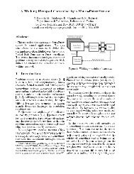
Fig. 2.<br />
Integrating <strong>Neuro</strong>-<strong>Fuzzy</strong> systems with FSA.<br />
ents by slightly changing network parameters and estimating<br />
the changes of the network error.<br />
E. Finite State Au<strong>to</strong>mata<br />
NNs and FSs alone are not sucient <strong>to</strong>cover all control<br />
requirements, since they intrinsically have no memory of<br />
the plant state, unless external feedback is applied (this<br />
refers mainly <strong>to</strong> FSs). That is why it was felt necessary<br />
<strong>to</strong> integrate those controllers with Finite State Au<strong>to</strong>mata<br />
(FSA). Such au<strong>to</strong>mata can keep track of the discrete plant<br />
states, and vary the controller parameters accordingly.<br />
As shown in gure 2, an FSA can be integrated with an<br />
analog-type controller (e.g., a NN, an FS, or a PID). The<br />
FSA receives as inputs both a number of discrete signals<br />
z from the plant (e.g., ON/OFF sensors,...) and a number<br />
of discrete signals z n obtained from thresholding some<br />
controller outputs (i.e., u > , with a programmable<br />
threshold).<br />
On the other hand, the FSA can both vary the controller<br />
parameters W ~ k (e.g., weight matrices, fuzzy rules, or PID<br />
parameters, etc.) and activateanumber of discrete actua<strong>to</strong>rs<br />
s (if any). In practice it is possible <strong>to</strong> dene a set of<br />
controller parameters for each of the discrete states of the<br />
au<strong>to</strong>ma<strong>to</strong>n. States can also appear in the antecedents of<br />
the fuzzy rules.<br />
Several plants may have many dierent states, according<br />
<strong>to</strong> operating conditions. Examples are: the dierent<br />
strokes of strongly non-linear trajec<strong>to</strong>ries, control of robot<br />
arms with dierent load conditions; forward and backward<br />
steps of walking robots; optimal operation of <strong>to</strong>oling machines<br />
with dierent <strong>to</strong>ols; etc.<br />
Instead of using an FSA interacting with a set of simpler<br />
controllers, plants with well-dened states might also be<br />
controlled by a single but more complex controller with<br />
memory. The advantages of the FSA-based solution are<br />
the following:<br />
1. the overall controller is subdivided in<strong>to</strong> a set of simpler<br />
controllers; each of these may often be as simple<br />
as a linear controller;<br />
2. each controller will be trained only over a limited subset<br />
of the state space;<br />
3. controllers can be trained independently of each other,<br />
therefore training one of them does not aect any of<br />
the others;
4. each controller has a reduced size and can be implemented<br />
in an optimal way, also by using dierent<br />
paradigms for each one (e.g., FSs, NNs, PIDs, etc.).<br />
Unfortunately, traditional FSA interacting with neurofuzzy<br />
controllers have few major drawbacks:<br />
1. The overall controller characteristic may change<br />
abruptly when the FSA has a state transition. This<br />
may often cause very high accelerations and jerks<br />
which may increase mechanical stresses, vibrations,<br />
and often reduce comfort and possibly also lifetime<br />
of the plant.<br />
2. To reduce discontinuities, either an additional<br />
\smoothing" subsystem is needed (but this often worsens<br />
the overall system performance), or the individual<br />
controllers should be designed <strong>to</strong> take care of state<br />
changes (but this increases the complexity and the duration<br />
of training).<br />
Section IV-A describes <strong>Fuzzy</strong> State Au<strong>to</strong>mata, which are<br />
an alternative solution <strong>to</strong> the problems listed above. They<br />
are derived from the tight integration of neuro-fuzzy systems<br />
and traditional FSA, but they have better performance<br />
and are more suited <strong>to</strong> design smooth characteristics<br />
and <strong>to</strong> deal with sequences of events.<br />
III. Comparison<br />
An HIC can be designed by combining one or more of<br />
the above mentioned paradigms, in a large variety of possibilities.<br />
The designer of a HIC can choose among several<br />
paradigms according both <strong>to</strong> system requirements and <strong>to</strong><br />
what form of knowledge he has about the plant. Anyway,<br />
some general considerations can be drawn <strong>to</strong> help a designer<br />
choose the best paradigm.<br />
A. Neural Networks<br />
The two major features of neural networks are massive<br />
parallel processing and adaptivity. By virtue of the distributed<br />
nature of information in the network, a neural<br />
network has the following properties:<br />
Fault <strong>to</strong>lerance. If some neurons are destroyed or accidentally<br />
disabled, then the output remains virtually<br />
unaected. At the most, the network's performance<br />
degrades gracefully rather than failing in a<br />
catastrophic way. This makes neural networks extremely<br />
well-suited <strong>to</strong> applications where failure of<br />
control equipment has catastrophic consequences.<br />
Flexibility. A large varietyofnetwork <strong>to</strong>pologies can be<br />
chosen, where each neuron may act as an independent<br />
processing and distribution center of information for<br />
the neural network.<br />
VLSI Implementability. Neural networks can be implemented<br />
in silicon using analog VLSI, resulting in<br />
very high-speed processing which is ideal for real-time<br />
control.<br />
Adaptivity. Adjusting its synaptic weights in an orderly<br />
fashion, a neural network can adapt <strong>to</strong> changes<br />
in the surrounding environment, or in the plant characteristics,<br />
showing its ability <strong>to</strong> learn and generalize.<br />
Generalization means <strong>to</strong> yield reasonable outputs for<br />
inputs not included in the training set.<br />
Nevertheless, NNs and also FSs have a big drawback<br />
which limits their applicability <strong>to</strong> critical systems; in practice,<br />
it is almost impossible <strong>to</strong> guarantee the behavior of a<br />
network in presence of input stimuli which were not presented<br />
during training. Because of that, the response of the<br />
network <strong>to</strong> unforeseen conditions (e.g., particular faults or<br />
operating conditions) cannot be predicted.<br />
Neural networks can be low-level model-free estima<strong>to</strong>rs,<br />
that is their design is based directly on real data with no<br />
need for an analytical mathematical model of the underlying<br />
system. This implies that neural networks are ideal for<br />
control of non-linear or complex systems.<br />
Knowledge about the environment in which a neural network<br />
is supposed <strong>to</strong> operate consists of two kinds of data,<br />
namely, prior information which corresponds <strong>to</strong> known<br />
facts or properties of the underlying system, and numeric<br />
measurements of input/output variables which are typically<br />
obtained by means of sensors (training set).<br />
Up <strong>to</strong> now, there is no way <strong>to</strong> map directly a priori \linguistic"<br />
knowledge (like that provided by ahuman expert)<br />
on<strong>to</strong> a neural network. Nevertheless, prior knowledge can<br />
partially be exploited <strong>to</strong> design a neural network with a<br />
specialized structure, i.e., a network with local connections<br />
between neurons or weight sharing [3].<br />
A neural network acquires knowledge usually from samples<br />
through a learning process. Back-propagation is by<br />
far the most used training algorithm in feed-forward neural<br />
networks thanks <strong>to</strong> its eectiveness and relative easiness<br />
of application.<br />
Independently of the learning algorithm used, the training<br />
process is very time-consuming, and this time increases<br />
typically with the number of hidden layers and the number<br />
of neuron per hidden layer. Anyway, itisworth <strong>to</strong> recall<br />
that a neural network is a massive parallel device and, even<br />
if training is time-consuming, in successive control operation<br />
a high throughput can be easily achieved (this applies<br />
only when dedicated hardware implementations are used;<br />
see also section V).<br />
In control applications, neural networks can be used according<br />
<strong>to</strong> the following strategies.<br />
Neural controllers with o-line training. A neural network<br />
can be trained <strong>to</strong> duplicate another (linear or<br />
non-linear) controller, which is used <strong>to</strong> generate an appropriate<br />
training set. In this case the neural network<br />
usually has state feedback.<br />
Passive learning neural controllers. The neural network<br />
learns directly from the plant, by on-line minimization<br />
of an appropriate cost function (often the<br />
square sum of errors). Actually, the controller behaves<br />
more as an adaptive than as a learning controller [1]<br />
because of possible over-tting around the actual trajec<strong>to</strong>ries<br />
in the state space.<br />
Active learning neural controllers. The neural network<br />
learns directly from the plant, as in the previous case.<br />
However, it tries also <strong>to</strong> learn from untrained regions<br />
in the state space, thus improving overall performance
+<br />
-<br />
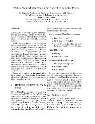
Fig. 3.<br />
Input pattern<br />
Genera<strong>to</strong>r<br />
PID<br />
Inverse<br />
Network<br />
Plant<br />
Canceling non-linearities with a trained NN.<br />
Fig. 4.<br />
Inverse<br />
Network<br />
Backpropagation<br />
Trainer<br />
Model<br />
Network<br />
Generation of an inverse network.<br />
for rapidly varying plant conditions or for unforeseen<br />
input conditions.<br />
Inverse controllers. The neural network learns the inverse<br />
transfer function of the plant. The inverse network<br />
can then be used either alone as an open loop<br />
controller or, better, <strong>to</strong> linearize (at least partially)<br />
a plant in a closed loop control architecture (see gure<br />
3).<br />
The inverse model of the plant can be obtained by<br />
training a neural network <strong>to</strong> generate plant inputs<br />
when fed with the corresponding outputs. Alternatively,<br />
a rst neural network is trained <strong>to</strong> implement<br />
the direct plant characteristic, then a second neural<br />
network is trained <strong>to</strong> model the inverse relation of the<br />
former (see gure 4).<br />
The main criticism against neural networks is that they<br />
act as black boxes so that it is dicult <strong>to</strong> gain insight in<strong>to</strong><br />
their operation, mainly with respect <strong>to</strong> the dynamics of<br />
the learning process. Furthermore, as no specic physical<br />
meaning can be associated with the adjustable parameters<br />
of the back-propagation algorithm, they are usually set <strong>to</strong><br />
random initial values with negative consequences on the<br />
training time.<br />
B. <strong>Fuzzy</strong> Systems<br />
While neural networks mimic the brain architecture,<br />
fuzzy logic simulates human approximate reasoning. Like<br />
neural networks, fuzzy systems can model general nonlinear<br />
processes. Unlike neural networks, however, fuzzy<br />
systems provide qualitative description of system properties<br />
and behavior, thus allowing both an easy exploitation<br />
of available a priori knowledge provided by human experts,<br />
and a clear insight in<strong>to</strong> system operation. In fact, the<br />
variables of the system (i.e., measured variables and control<br />
variables) are considered as linguistic variables (represented<br />
by fuzzy sets with suitably chosen membership<br />
functions) and system behavior is described in terms of logical<br />
relationships (represented by IF-THEN rules) between<br />
such variables.<br />
<strong>Fuzzy</strong> systems provide a natural framework for expressing<br />
vague, uncertain or imprecise knowledge which is intrinsic<br />
in most plant models, so that human operating experience<br />
can be easily exploited.<br />
<strong>Fuzzy</strong> systems are high-level model-free estima<strong>to</strong>rs.<br />
They turn out <strong>to</strong> be simple <strong>to</strong> design, easy <strong>to</strong> set up and <strong>to</strong><br />
inspect, thanks <strong>to</strong> their logical structure and step-by-step<br />
procedures. It is also possible <strong>to</strong> modify some parts of a<br />
fuzzy system (e.g., some rules or membership functions)<br />
and have a reasonable idea of the eect of such changes.<br />
In this way one can develop a fuzzy system in a heuristic<br />
manner obtaining a working system that can then be<br />
improved by an optimizing process (for instance, Genetic<br />
Algorithms, Simulated Annealing, etc.). Actually, a fuzzy<br />
system can be trained (i.e., the fuzzy rules can be au<strong>to</strong>matically<br />
generated) using any of several learning algorithms<br />
based on numerical information. For example, a fuzzy system<br />
can be represented as a feed-forward network, and its<br />
parameters can be adjusted using back-propagation training<br />
algorithms. This development methodology can prove<br />
eective <strong>to</strong> avoid the problem of local minima which is<br />
present in several optimization algorithms.<br />
Traditionally, a specic fuzzy system is developed by consulting<br />
human experts who are able <strong>to</strong> control the process<br />
manually and successfully, and who provide linguistic descriptions<br />
of both the plant and control actions. Such linguistic<br />
information can be directly and easily incorporated<br />
in<strong>to</strong> the fuzzy control rules. On the other hand, when a<br />
domain expert is not available, the necessary knowledge <strong>to</strong><br />
build the rule base has <strong>to</strong> be acquired by directly operating<br />
the process being controlled.<br />
The rules generated from input-output pairs may then<br />
possibly be combined with rules obtained in linguistic<br />
terms in<strong>to</strong> a unique fuzzy rule base [2], [6]. In this way,<br />
adaptive fuzzy systems can be built which integrate linguistic<br />
information (in the form of IF-THEN rules) and<br />
numerical information (in the form of input-output pairs).<br />
Let us note that the adjustable parameters of a fuzzy system,<br />
unlike neural networks, have precise physical meanings,<br />
as they represent centers and widths of the fuzzy sets<br />
in the antecedent and consequent of fuzzy rules. As a consequence,<br />
it is often possible <strong>to</strong> choose appropriate initial<br />
values for such parameters thus providing a good starting<br />
point for the training algorithm, which results in higher<br />
convergence [2].<br />
By exploiting the intrinsic capabilities of fuzzy logic of<br />
converting human expertise in a set of linguistic rules, and<br />
<strong>to</strong> provide adaptivity and robust performance under changing<br />
operating conditions, fuzzy systems are able <strong>to</strong> characterize<br />
and control a system whose model is not known,<br />
ill-dened, or has parameter variation problems.<br />
<strong>Fuzzy</strong> systems can be implemented using conventional<br />
microprocessors with A/D and D/A converters or can be<br />
realized directly as analog devices.<br />
When the plant is very complex, the set of fuzzy rules<br />
may result unmanageable since the number of rules depends<br />
exponentially on the number of system variables. In<br />
this case, a hierarchical fuzzy controller can be used, which<br />
consists in a \cascade" of traditional fuzzy controllers [10].<br />
More precisely, the system variables are classied based<br />
on their importance, and the rules in the n th level are
expressed in terms of both the system variables of the<br />
n th class, and the output of the rule set in the previous<br />
level [10]. This approach makes the <strong>to</strong>tal number of rules<br />
a nearly linear function of the system variables.<br />
In spite of the aforementioned advantages, however, it<br />
should be pointed out that major limitations of fuzzy controllers<br />
are the lack of a general systematic procedure for<br />
au<strong>to</strong>matic rule learning and tuning, and the lack of assessed<br />
criteria for determining the best shape of membership functions,<br />
their degree of overlapping, and the partitions of the<br />
input and output spaces.<br />
Wrong membership functions, for example, can lead <strong>to</strong><br />
poor controller performance and possibly <strong>to</strong> instability [1].<br />
C. <strong>Neuro</strong>-<strong>Fuzzy</strong> Systems<br />
Neural networks and fuzzy systems can essentially be applied<br />
<strong>to</strong> solve the same problems. As they have dierent<br />
advantages and drawbacks, it is quite reasonable <strong>to</strong> consider<br />
the possibility ofintegrating the two paradigms in<strong>to</strong><br />
the same system in order <strong>to</strong> benet from both of them.<br />
An important connection between neural networks and<br />
fuzzy systems is that both of them are universal approxima<strong>to</strong>rs,<br />
i.e., they are capable of approximating any real continuous<br />
function on a compact set <strong>to</strong> an arbitrary accuracy.<br />
It follows that neural networks and fuzzy systems can approximate<br />
each other. This means that, on one hand, once<br />
a fuzzy controller has been dened, tested (and possibly<br />
tuned), an equivalent neural network can be trained until<br />
the desired accuracy has been reached. On the other hand,<br />
a neural controller can be approximated by an appropriate<br />
fuzzy controller, thus allowing a linguistic interpretation of<br />
the knowledge that the neural network has acquired from<br />
examples.<br />
Various ways of implementing fuzzy controllers by neural<br />
networks and various fuzzications of neural networks have<br />
been proposed in the literature. An ecient neuro-fuzzy<br />
paradigm is WRBF, described in section II-C, which in fact<br />
represents a unication algorithm between MLPs, RBFs<br />
and FSs.<br />
The basic reason for resorting <strong>to</strong> neuro-fuzzy paradigms<br />
is the following. As previously stated, the fundamental difference<br />
between fuzzy systems and neural networks is that<br />
the former are capable of incorporating linguistic information<br />
from human experts in a systematic way, whereas the<br />
latter are not. It follows that, in all those situations in<br />
which, in spite of a high degree of complexity and uncertainty,<br />
a real-world system is successfully controlled by<br />
skilled human opera<strong>to</strong>rs, a fuzzy controller is the most appropriate<br />
choice. This happens, for instance, in chemical<br />
processes, aircraft, etc. On the other hand, when a large<br />
amount of samples measured directly from the controlled<br />
plant are available, a neural controller may be more appropriate.<br />
Approximating fuzzy systems by neural networks allows<br />
exploitation of the inherent capability of neural networks <strong>to</strong><br />
perform massive parallel processing of information. This is<br />
of the utmost importance in all those applications in which<br />
large numbers of fuzzy rules have <strong>to</strong> be processed in realtime.<br />
In particular, the neural version of the fuzzy system<br />
can be run on hardware neural processors, when these are<br />
available and cheaper than other processors.<br />
A further benet from giving a numerical interpretation<br />
<strong>to</strong> the knowledge explicitly contained in a set of fuzzy rules<br />
is <strong>to</strong> allow numerical optimization (for instance, by means<br />
of s<strong>to</strong>chastic or genetic algorithms) of a set of fuzzy rules.<br />
Note also that mapping a fuzzy controller in<strong>to</strong> a neural<br />
network allows us <strong>to</strong> use human expertise <strong>to</strong> start learning<br />
from a point in the parameter space which is not far from<br />
the optimum, thus reducing the training time. Later, the<br />
optimized neural system may possibly be converted back<br />
in<strong>to</strong> an optimized fuzzy system.<br />
Finally, the learning capability of neural networks could<br />
be used for both building membership functions from sample<br />
data and ne-tuning the rule base, thus helping <strong>to</strong> solve<br />
some typical problems of fuzzy systems.<br />
Approximating neural networks by fuzzy systems allows<br />
<strong>to</strong> interpret in linguistic terms the knowledge hidden within<br />
the network internal parameters. This is useful in several<br />
applications, for example when the neural network has been<br />
trained <strong>to</strong> approximate a function or <strong>to</strong> model an unknown<br />
system. The knowledge acquired can then be transformed<br />
in<strong>to</strong> a linguistic form for later use, either by humans <strong>to</strong><br />
understand the phenomena, or by computers in articial<br />
intelligence <strong>to</strong>ols.<br />
Another application of fuzzy interpretation of neural matrices<br />
is <strong>to</strong> run neural networks on hardware fuzzy processors,<br />
when these are available and cheaper than other<br />
processors.<br />
IV. Recurrent Models<br />
A feed-forward neural network trained with the standard<br />
back-propagation algorithm implements a static inpu<strong>to</strong>utput<br />
mapping. However, in many real-world situations,<br />
such as signal processing, mo<strong>to</strong>r control, etc., temporal processing<br />
is usually involved. In such cases recurrent neural<br />
networks may be used, which have feedback connections<br />
from their outputs <strong>to</strong> their inputs <strong>to</strong> model the s<strong>to</strong>rage of<br />
temporal information. A recurrent network is capable of<br />
s<strong>to</strong>ring internal states and implementing complex dynamical<br />
functions.<br />
As in the case of feed-forward networks, error-correction<br />
learning techniques can be used <strong>to</strong> train recurrent networks,<br />
with the major dierence being that the input and output<br />
vec<strong>to</strong>rs are time sequences.<br />
A specic learning technique is Back-propagation<br />
Through Time (BTT), which is a generalization of the<br />
standard back-propagation [3]. BTT is based on \unfolding"<br />
a recurrent network in time <strong>to</strong> produce an equivalent<br />
multi-layer feed-forward network. More precisely, for<br />
sequences of maximum length T, the equivalent network<br />
is obtained by adding a new layer at each time step, so<br />
that the T-step forward operation of the recurrent network<br />
gives origin <strong>to</strong> a T-layered feed-forward network. The standard<br />
back-propagation algorithm is then applied <strong>to</strong> the<br />
unfolded network, considering that all copies of the \unfolded"<br />
weights must be identical, and the desired response
vec<strong>to</strong>r is associated with every copy of the output layer.<br />
By virtue of its capability of being both a sequence recognizer<br />
and a sequential pattern genera<strong>to</strong>r, a recurrent network<br />
can be used as a non-linear controller of a dynamical<br />
system. Indeed, based on a model of the system <strong>to</strong> be<br />
controlled, sequences of system internal states can be input<br />
in<strong>to</strong> the network, so that the network output at any<br />
given time depends on network previous states as well as<br />
on the current input. The network can then be trained using<br />
BTT, for instance, <strong>to</strong> maximize some utility function<br />
over a time period.<br />
A. <strong>Fuzzy</strong> State Au<strong>to</strong>mata<br />
As anticipated in section II-E, neuro-fuzzy control methods<br />
can also be used in conjunction with traditional FSA<br />
<strong>to</strong> deal with the dierent plant states, for the following<br />
reasons:<br />
1. fuzzy logic allows <strong>to</strong> include the available \human<br />
knowledge" in<strong>to</strong> the solution of a problem [2], but is<br />
not well suited <strong>to</strong> deal with sequences of events;<br />
2. FSA are ideally suited <strong>to</strong> deal with sequences of<br />
events, but they are not good at handling continuous<br />
signals and human knowledge;<br />
3. fuzzy systems are generally feed-forward systems,<br />
without feedback, as fuzzy logic is mostly associated<br />
with memoryless systems. This is because no method<br />
has been found so far <strong>to</strong> describe recurrent fuzzy systems<br />
eciently;<br />
4. mixing neuro-fuzzy systems with FSA allows <strong>to</strong> include<br />
human knowledge and training capabilities in<strong>to</strong><br />
recurrent systems (namely, with memory) which can<br />
therefore deal with sequences of events, dierent plant<br />
states, etc.<br />
Unfortunately, neuro-fuzzy systems associated with FSA<br />
have the drawbacks described in section II-E; these drawbacks<br />
can be reduced by using the <strong>Fuzzy</strong> State Au<strong>to</strong>mata<br />
described further.<br />
The main dierence of <strong>Fuzzy</strong> State Au<strong>to</strong>mata (FFSAs)<br />
with respect <strong>to</strong> traditional FSA is that transitions in fuzzy<br />
au<strong>to</strong>mata are not triggered by crisp events but by fuzzy<br />
variables, and state transitions are fuzzy as well. It immediately<br />
results that, at any time, the whole system is<br />
not necessarily in one and only one well-dened state, but<br />
it may well be in more states at the same time, each one<br />
associated with its own membership value.<br />
State transitions are therefore smoother and slower, even<br />
if the controllers activated by each state are not designed<br />
<strong>to</strong> smooth the transitions. As a consequence, all the individual<br />
controllers may become as simple as a traditional<br />
PID, each one designed for a dierent target specic <strong>to</strong><br />
that state. The FFSA then takes care of smoothing discontinuities<br />
between partial local characteristics, but the<br />
overall system is much simpler <strong>to</strong> design and tune than a<br />
traditional controller with similar characteristics.<br />
Unfortunately FFSA have a drawback, that is, as the<br />
au<strong>to</strong>mata are often in more than one state, they have <strong>to</strong><br />
process more than one controller at any time. This increase<br />
of computing time often counterbalance the higher speed<br />
SA<br />
CA<br />
x is NOT A<br />
SC<br />
CC<br />
x is A<br />
x is C<br />
SB<br />
CB<br />
x is D<br />
SD<br />
CD<br />
x is B<br />
Fig. 5. An example of an FFSA. S j are state names, while C j are<br />
controllers associated with each state.<br />
that can be achieved through the use of simpler controllers.<br />
In practice, FFSA achieve approximately the same speed<br />
as traditional FSA controlling neuro-fuzzy controllers, but<br />
they are easier <strong>to</strong> design (especially for complex systems)<br />
and produce smoother trajec<strong>to</strong>ries.<br />
So far, the theory of FFSA has been tested on some<br />
applications in the eld of control, for instance <strong>to</strong> design<br />
the Motion and Leg Coordination <strong>Control</strong>s of the walking<br />
hexapode described in section VI-C, where FFSA have<br />
been used as a way <strong>to</strong> specify the cooperation between individual<br />
legs. This example is shortly described in section VI.<br />
As shown in gure 5, an FFSA looks very similar <strong>to</strong> a<br />
traditional FSA, in the sense that it can be represented as a<br />
collection of fuzzy states S j (namely, the circles), connected<br />
by fuzzy transitions (namely, the arrows). Each fuzzy transition<br />
is labeled by a fuzzy expression which can be as complex<br />
as desired (A, B, C, D are traditional fuzzy sets).<br />
As in a traditional FSA, a state represents uniquely the<br />
operating conditions of an FFSA, at any given instant.<br />
But, unlike FSA, a system need not be in only one state at<br />
a time. Each state S j is therefore associated with a fuzzy<br />
state activity Sj 2 [0; 1], which represents \how much"<br />
the system is in that particular state. The state activity is<br />
somehow equivalent <strong>to</strong> the degree of membership of a fuzzy<br />
variable, yet note that the state in an FFSA is not a fuzzy<br />
variable.<br />
If we associated a state activity with states in a traditional<br />
FSA, it would be:<br />
Sj =<br />
1; for the active state<br />
0; for all other states<br />
X<br />
with the constraint that the <strong>to</strong>tal activity:<br />
j<br />
(8)<br />
Sj =1; (9)<br />
meaning that the system is always in one and only one<br />
well dened state S j (the one with Sj<br />
= 1) and in no<br />
other state.<br />
Constraint (9) also applies <strong>to</strong> FFSA, therefore activity<br />
can be distributed among several states and can partially<br />
move from one state <strong>to</strong> another (possibly more than one),<br />
but the <strong>to</strong>tal activity shall always be constant.<br />
FFSA can be of dierent types [7]: time-independent and<br />
time-dependent; the former can either be synchronous or<br />
asynchronous, which somewhat reects synchronous and
asynchronous FSA, respectively. They dier only in the<br />
way state activity moves from one state <strong>to</strong> another, according<br />
<strong>to</strong> the degrees of membership of the fuzzy transitions.<br />
We could roughly say that:<br />
in asynchronous, time-independent FFSA, state transitions<br />
may take place as soon as inputs vary (yet transitions<br />
are not so abrupt as in traditional FSA);<br />
in synchronous, time-independent FFSA, state transitions<br />
are computed in a way similar <strong>to</strong> asynchronous<br />
FFSA, but they are applied only at the next clock cycle;<br />
in time-dependent FFSA, there is always an intrinsic<br />
delay (usually larger than the clock period, if any)<br />
between input variations and the corresponding state<br />
transitions.<br />
Furthermore, each state S j is associated with a dierent<br />
controller Y ~ = C j ( X) ~ (each controller can independently<br />
be an FS, a NN, a linear controller, etc.). The overall<br />
characteristic of the FFSA controller is given by the average<br />
of all C j weighted by the corresponding state activities:<br />
Fig. 6.<br />
Parameters of specialized<br />
neuro-fuzzy controllers<br />
<strong>Neuro</strong>-<strong>Fuzzy</strong><br />
<strong>Control</strong>lers<br />
Selec<strong>to</strong>r<br />
Finite State<br />
Au<strong>to</strong>ma<strong>to</strong>n<br />
<strong>Neuro</strong>-<strong>Fuzzy</strong><br />
Processor<br />
(AMINAH)<br />
Sensors<br />
Actua<strong>to</strong>rs<br />
Plant discrete states<br />
Plant<br />
Working principle of the proposed controller architectures.<br />
~Y = X j<br />
Sj C j ( ~ X) (10)<br />
Further details on FFSA can be found in [7].<br />
V. Hardware Implementations<br />
Real-time control of non-linear plants [1], [14] is often a<br />
hard and computationally intensive task.<br />
The availability of dedicated neuro-fuzzy processors permits<br />
a very fast implementation of neuro-fuzzy algorithms,<br />
and therefore it allows <strong>to</strong> use these methods in real-time<br />
applications, where a high sampling rate (namely, >1kHz)<br />
is required. The drawback is the reduced exibility of the<br />
system due <strong>to</strong> the rigid architecture of the dedicated neurofuzzy<br />
processors.<br />
On the other side, if a great exibility is required, several<br />
solutions can be envisaged, ranging from general purpose<br />
DSPs <strong>to</strong> commercial fuzzy inference processors.<br />
We developed a control system, DANIELA (Digital Analog<br />
<strong>Neuro</strong>-fuzzy Interface for Enhanced Learning Applications),<br />
a real-time neuro-fuzzy controller that implements<br />
intelligent control algorithms mixing neuro-fuzzy<br />
paradigms with Finite State Au<strong>to</strong>mata (FSA) [5] (see gure<br />
6).<br />
This mixing allows the system <strong>to</strong> change the control<br />
strategy according <strong>to</strong> the actual state of the plant (the<br />
FSA chooses one of the possible controllers). Our system<br />
uses specialized controllers for every dierent plant state.<br />
In order <strong>to</strong> build a pro<strong>to</strong>type of this system we developed<br />
a cus<strong>to</strong>m <strong>Neuro</strong>-<strong>Fuzzy</strong> Processor called AMINAH [13], that<br />
implements several neural paradigms and/or fuzzy systems.<br />
This new chip, which is the evolution of a previous neural<br />
processor [5], uses Coherent Pulse Width Modulation<br />
(CPWM) for low-power computation [5] and also <strong>to</strong> interface<br />
the controller with sensors and eec<strong>to</strong>rs of the system.<br />
As shown in gure 7, DANIELA is mainly composed of a<br />
<strong>Neuro</strong>-<strong>Fuzzy</strong> Processor (AMINAH) [13] that interacts with a<br />
Fig. 7.<br />
Pro<strong>to</strong>type of the controller board.<br />
general purpose 68HC11 microcontroller and a memory in<br />
order <strong>to</strong> control the plant. Other important parts of the<br />
system are Analog <strong>to</strong> Digital converters, a Conguration<br />
and Refresh block and a Host Interface block. DANIELA<br />
has also special Power Drivers used <strong>to</strong> drive the actua<strong>to</strong>rs<br />
in the plant.<br />
Plant control is realized with a neuro-fuzzy algorithm<br />
computed by the neuro-fuzzy processor. Algorithm characteristics<br />
both for neural and fuzzy systems are dened<br />
by a matrix of synaptic weights and other parameters that<br />
are s<strong>to</strong>red in<strong>to</strong> the neuro-fuzzy processor.<br />
In order <strong>to</strong> dene dierent control strategies (optionally,<br />
one per each state of the FSA) there are dierent matrices of<br />
synaptic weights and parameters s<strong>to</strong>red in as many memory<br />
banks of the weight memory.<br />
Only one bank can be active at any time and its data<br />
are transferred <strong>to</strong> the internal memory of the neuro-fuzzy<br />
processor by the Conguration and Refresh Block every<br />
time the FSA changes state.<br />
This memory organization allows <strong>to</strong> obtain dierent neural<br />
controllers just by changing the active memory bank.<br />
Weight memory is also used <strong>to</strong> s<strong>to</strong>re tables of FSA states<br />
and outputs; these parameters are used by the microcontroller<br />
<strong>to</strong> implement the FSA controller.<br />
The microcontroller performs the following tasks:<br />
On-line training: by sampling neuro-fuzzy inputs and<br />
outputs (also hidden units) and modifying matrices of<br />
synaptic weights s<strong>to</strong>red in<strong>to</strong> the weight memory [1],
[14]. As the microcontroller is less powerful than the<br />
neural chip, learning is a relatively slow process, but<br />
this is not a problem in most learning controllers.<br />
FSA controller: by tracking the discrete states of the<br />
plant and selecting a suitable memory bank in order<br />
<strong>to</strong> change the control strategy. The computational<br />
requirements for the FSA are less stringent, as in most<br />
plants state transitions are much less frequent than<br />
neural computations.<br />
Board self test: performing tests and diagnostics at<br />
power up.<br />
Interface with a host computer, which can either write<br />
data in<strong>to</strong> the memory or read several debugging information<br />
from the microcontroller (such as neural states,<br />
learning performance, actual FSA state, etc.).<br />
<br />
<br />
<br />
In DANIELA, these tasks are performed by the 68HC11;<br />
a DSP-based version of this control system is also under<br />
development.<br />
In the pro<strong>to</strong>type board of the DANIELA system, a 16Kbyte<br />
RAM is used as weight memory and contains 16 memory<br />
blocks; each block consists of 512 bytes of synaptic<br />
weights (8 bit/weight) and other neural parameters<br />
(about 500 bytes), resulting in 1Kbyte per weight matrix.<br />
Most of the other logic circuits are implemented on an<br />
ALTERA EPM7128 c .<br />
This pro<strong>to</strong>type board includes also A <strong>to</strong> D converters<br />
and power switching ampliers for mo<strong>to</strong>r driving.<br />
The host programming interface is realized under<br />
MATLAB c where several cus<strong>to</strong>m C++ classes and routines<br />
are used <strong>to</strong> download and receive data <strong>to</strong>/from<br />
DANIELA.<br />
We also developed, in collaboration with the Department<br />
of Au<strong>to</strong>matic and Computer Science, a new dedicated<br />
MATLAB <strong>to</strong>olbox (MatDSP), where specialized functions<br />
allow <strong>to</strong> integrate commercial DSPs and cus<strong>to</strong>m <strong>Neuro</strong>-<br />
<strong>Fuzzy</strong> processors with the MATLAB computing environment.<br />
From the user point of view, this new <strong>to</strong>olbox allow <strong>to</strong><br />
directly use the DSP <strong>to</strong> acquire data, perform signal processing<br />
and run xed structure controllers. If required by<br />
the implemented algorithm, the DSP can directly use a<br />
<strong>Neuro</strong>-<strong>Fuzzy</strong> computing core (AMINAH), just supervising<br />
the system like the 68HC11 in DANIELA.<br />
VI. Application Examples<br />
This section describes three applications of the proposed<br />
methodology. The rst one, a vacuum roll coating machine,<br />
is a simple but practical problem, which can be solved with<br />
few fuzzy rules acquired from a human expert; the second<br />
one, a bidimensional inverted pendulum in polar coordinates,<br />
is a quite <strong>to</strong>ugh problem, which can be solved<br />
by means of a hierarchical hybrid neuro-fuzzy-linear approach,<br />
using only feed-forward networks; the third one,<br />
the motion coordination and control of a six-legged walking<br />
hexapode, is another complex problem which has been<br />
solved by means of recurrent <strong>Fuzzy</strong> State Au<strong>to</strong>mata.<br />
Fig. 8.<br />
Vacuum<br />
Film Rollers<br />
Aluminium<br />
Sources<br />
Film coating oven.<br />
Film under<br />
Coating<br />
A. Process <strong>Control</strong> in Vacuum Roll Coating Machines<br />
A vacuum roll coating machine (sketched in gure 8)<br />
deposits a thin layer of material (usually aluminum) on a<br />
substrate. The substrate is a lm of polyester (or, in some<br />
cases, paper) which is unrolled from a drum and passes<br />
over a series of liquid aluminum pools (sources), where it<br />
collects the aluminum vapor; then it is rolled up again by<br />
a second drum. Once the vacuum condition has been established<br />
inside the metallization chamber, the fac<strong>to</strong>rs affecting<br />
the thickness and the quality of the deposition are<br />
the speed of the lm, the temperature of the sources and<br />
the feeding rate of aluminum in<strong>to</strong> the sources. It is of primary<br />
importance <strong>to</strong> adjust the power of the sources as a<br />
function of the aluminum rate, in order <strong>to</strong> avoid spitting<br />
and, consequently, pin windows in the lm [11].<br />
The metallization process is usually controlled by skilled<br />
opera<strong>to</strong>rs. This means that there is an eect on the quality<br />
of the results, depending on the dierent opera<strong>to</strong>r procedures,<br />
in such a way that the idea of au<strong>to</strong>mating the<br />
control of the process is very attractive, both <strong>to</strong> achieve<br />
independence from opera<strong>to</strong>r and <strong>to</strong> obtain better overall<br />
quality. On the other hand, given the high non-linearity<br />
of the evaporation process, the change in the characteristics<br />
of the sources (due <strong>to</strong> the erosion phenomena caused<br />
by liquid aluminum), and the change in the metal collection<br />
eciency, it is very dicult <strong>to</strong> establish an optimal<br />
mathematical model for the controller of the metallization<br />
process.<br />
The problem can then be tacked with the help of fuzzy<br />
logic, by transferring the knowledge of the opera<strong>to</strong>r <strong>to</strong> a<br />
set of rules based on linguistic variables. Based on these<br />
considerations, we decided <strong>to</strong> implement a fuzzy controller<br />
<strong>to</strong> be tested on the machine. The controller was developed<br />
under the form of software <strong>to</strong> be run on a microcontroller.<br />
After the plant simula<strong>to</strong>r showed <strong>to</strong> perform in accordance<br />
with the real plant, the fuzzy controller was developed,<br />
based on three inputs (state of the aluminum pool,<br />
evaporation condition, and optical density (thickness) of<br />
the deposition) and two outputs (aluminum feeding rate<br />
and heating power). The two outputs are generated by<br />
means of 5 and 25 rules, respectively. <strong>Control</strong>ler parameters<br />
were rst chosen according <strong>to</strong> the opera<strong>to</strong>r's experience
and <strong>to</strong> the general knowledge of the involved phenomena,<br />
and then optimized by means of a genetic optimizer, where<br />
the tness indica<strong>to</strong>r was the settling time after a disturbance.<br />
At the end of the development process, the controller<br />
was installed on the real coating machine for the nal re-<br />
nement of the parameters and for a phase of thorough<br />
testing of its behavior. The rst results were very good in<br />
terms of uniformity of the metallization (uniformity better<br />
than 5% was achieved), and we expect a longer life of the<br />
sources as a result of the improved quality of the control.<br />
B. Inverted Pendulum in Polar Coordinates<br />
A typical application used <strong>to</strong> test the eectiveness of<br />
fuzzy controllers is the inverted pendulum, a well known<br />
unidimensional non-linear system [12]. A natural extension<br />
of this application is the bidimensional inverted pendulum,<br />
which consists of a pole, with a mass on <strong>to</strong>p, suspended by<br />
a spherical joint onamoving base (the case of a distributed<br />
mass is analogous).<br />
In the examined problem, the base is provided with two<br />
powered wheels. The base can either move <strong>to</strong> and fro, or<br />
turn around the vertical axis, but cannot slide sideways.<br />
It is important <strong>to</strong> point out that the control of this simple<br />
system can be challenging, because when the pendulum<br />
tends <strong>to</strong> fall perpendicularly <strong>to</strong> the current base heading<br />
the base has <strong>to</strong> rotate before being able <strong>to</strong> eectively act<br />
on the pendulum movement. Due <strong>to</strong> the operation in polar<br />
coordinates, the system is intrinsically ill-conditioned, unstable<br />
and its characteristic has a large discontinuity when<br />
the pole is nearly vertical.<br />
The pendulum is suspended on the base with a joystick,<br />
which provides position information <strong>to</strong> the controller, in<br />
the form of two angular coordinates, x and y (the two<br />
projections of the angle between the pole and the vertical<br />
axis).<br />
The fuzzy inference system which generates control information<br />
for the force is developed through a hierarchical<br />
approach. First of all, we will take in<strong>to</strong> account the case<br />
in which the pendulum falls in (or near) the heading direction;<br />
in such case recovery is possible by moving the base in<br />
the same direction as the falling pendulum. In particular<br />
we control the pendulum with a modied PID controller<br />
(actually a PD, since there is no integral term):<br />
F = pid(; x )=k p sign( x )+k d<br />
d<br />
dt x (11)<br />
where F is the <strong>to</strong>tal force applied <strong>to</strong> the wheels.<br />
To improve system performance, the PD controller de-<br />
ned by (11) can be replaced by a non-linear controller<br />
described by the following fuzzy rules:<br />
8<<br />
:<br />
IF is pos THEN F = pid(; x )+k o<br />
pid (; x )=<br />
IF is neg THEN F = pid(; x ) , k o<br />
(12)<br />
in which pos and neg are appropriate fuzzy sets, while k o<br />
is an appropriate bias force <strong>to</strong> improve response speed.<br />
Normalized Cost Function<br />
1.2<br />
1<br />
0.8<br />
0.6<br />
0.4<br />
0.2<br />
Simulated Annealing<br />
Weight Perturbation<br />
0<br />
0 10 20 30 40 50<br />
(steps)<br />
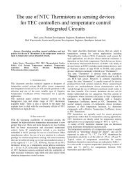
Fig. 9. Cost function decrease during optimization with simulated<br />
annealing and weight perturbation.<br />
Theta (degrees)<br />
Fig. 10.<br />
5<br />
4<br />
3<br />
2<br />
1<br />
Before Optimization<br />
After Optimization<br />
0<br />
0 50 100 150 200 250 300<br />
(1/100 sec)<br />
Eect of parameter optimization on pendulum stability.<br />
Instead, if the pendulum falls in a direction orthogonal<br />
(or almost orthogonal) <strong>to</strong> the current base heading, the<br />
applied force sign is reversed.<br />
This control action imposes a backwards movement <strong>to</strong><br />
the base which tends <strong>to</strong> move the pendulum closer <strong>to</strong> the<br />
heading direction, where it can be then better controlled.<br />
The selection between these two opposite control strategies<br />
depends on the angle between the heading direction and<br />
the projection of the pendulum on the horizontal plane<br />
( is converted in<strong>to</strong> the range (,=2;=2] rad by adding<br />
or subtracting rad). These two basic control techniques<br />
correspond <strong>to</strong> the following fuzzy rules (from (11)):<br />
IF is zero THEN F = pid (; x )<br />
IF is NOT zero THEN F = ,K Z pid (; x )<br />
where zero is a fuzzy set corresponding <strong>to</strong> a bell shaped<br />
membership function.<br />
An analogous hybrid fuzzy-PID controller evaluates the<br />
d<br />
control <strong>to</strong>rque T based on , and , which are all provided<br />
by a signal preprocessor.<br />
dt<br />
Finally, the actual forces applied <strong>to</strong> the two driving<br />
wheels are calculated from <strong>to</strong>tal force and <strong>to</strong>rque.<br />
The overall controller behavior depends on the values of<br />
several parameters, which describe both the shape of membership<br />
functions and the pid () response. These parameters<br />
were initially chosen with a heuristic method, based
POWER<br />
LEGANGLE is BACK<br />
LIFT<br />
BACK<br />
FRONT<br />
C1<br />
C2<br />
LEGHEIGHT is DOWN<br />
LEGHEIGHT is UP<br />
DOWN<br />
UP<br />
LEGANGLE (degrees)<br />
CONTACT<br />
LEGANGLE is FRONT<br />
RETURN<br />
VERY HIGH<br />
C4<br />
C3<br />
LEGSPEED is STILL<br />
LEGHEIGHT (mm)<br />
LEGANGLE is MORELESS FRONT<br />
AND<br />
TIMEOUT<br />
LEGHEIGHT is VERY HIGH<br />
BACKSTEP<br />
DELTA (LEGANGLE) is<br />
UPSTEP<br />
STILL<br />
C5<br />
FEWDEGREES<br />
C6<br />
LEGSPEED (degrees/sec)<br />
Fig. 12. <strong>Fuzzy</strong> State Au<strong>to</strong>ma<strong>to</strong>n for the leg controls of the walking<br />
hexapode.<br />
Fig. 11.<br />
The Hexapode Walking Machine.<br />
on a simple kinematic analysis, and then optimized, with<br />
respect <strong>to</strong> the standard deviation of , by means of both a<br />
weight perturbation method [3] and a simulated annealing<br />
algorithm. The evaluation of the cost function (standard<br />
deviation of ) was repeated at every optimization step for<br />
six dierent pendulum starting points in the phase space.<br />
Figure 9 reports the average cost function during the optimization<br />
process while gure 10 plots the initial transient<br />
of as a function of time before and after optimization.<br />
One can notice the stability improvement due <strong>to</strong> optimization.<br />
C. Hexapode Walking Machine<br />
Aim of the research is <strong>to</strong> design, build and test a small<br />
hexapode walking machine controlled by purposely developed<br />
neural chips, which can be used as a remotely controlled<br />
observation device and can evolve as a true mobile<br />
robot (see gure 11). The machine can also be used as<br />
an experimental test-bed for dierent control strategies <strong>to</strong><br />
investigate the possibility of small walking vehicles on different<br />
types of terrain.<br />
The main characteristics of the machine are: simple<br />
and lightweight mechanical architecture <strong>to</strong> contain overall<br />
costs, modularity <strong>to</strong> use the machine as a research <strong>to</strong>ol,<br />
exibility leading <strong>to</strong> the possibility of adapting the gait <strong>to</strong> a<br />
variety of terrains, possibility ofworking as an au<strong>to</strong>nomous<br />
system without the need of an umbilical cord for either energy<br />
supply or control.<br />
For these reasons, we chose <strong>to</strong> use low-cost permanent<br />
magnets electric mo<strong>to</strong>rs in connection with re-chargeable<br />
batteries and <strong>to</strong> adopt a gait in which the vehicle is always<br />
in conditions of static equilibrium. A "reptilian" stance<br />
is adopted as its energetic disadvantages are of small importance.<br />
The design chosen allows <strong>to</strong> assume an "insect"<br />
stance and even <strong>to</strong> switch <strong>to</strong> a quadruped "mammalian"<br />
conguration [15]. The mass of the mechanical components,<br />
including the electric mo<strong>to</strong>rs, is 24.3 Kg. The machine<br />
is already assembled and the rst tests are going on.<br />
Each leg is made of a shinbone and a thighbone both 50<br />
cm long; it has three degrees of freedom and is equipped<br />
with three current-controlled mo<strong>to</strong>rs. To obtain high e-<br />
ciency, switching ampliers are employed, which are perfectly<br />
matched with the CPWM encoding used in the DANIELA<br />
system (see section V). All the actua<strong>to</strong>rs are directly controlled<br />
by power drivers. One of the actua<strong>to</strong>rs must carry a<br />
signicant fraction of the hexapode weight (depending on<br />
the number of legs that support the body) and so its driver<br />
has a maximum output current of 20A (namely, 480W),<br />
while for the other two drivers the output current is only<br />
3A (namely, 72W).<br />
Since the control task is complex, the idea is <strong>to</strong> build<br />
a hierarchy of neuro-fuzzy controllers and FFSA. <strong>Neuro</strong>fuzzy<br />
controllers have been chosen because of their good<br />
behavior in the presence of non-linear systems and for their<br />
<br />
<br />
intrinsic generalization capability. The control system is<br />
organized in three dierent levels:<br />
Motion coordination control. It acts like a \central"<br />
controller, which gives the legs the right \highlevel"<br />
control signals (such as: robot speed, robot<br />
height from ground, radius of trajec<strong>to</strong>ry) <strong>to</strong> let the<br />
hexapode execute properly each gait. Obstacle avoidance<br />
is achieved by giving proper trajec<strong>to</strong>ry information<br />
<strong>to</strong> the individual leg controls. Only large obstacles<br />
are avoided, as small ones (namely roughness of<br />
the ground, small s<strong>to</strong>nes, holes, etc.) are handled by<br />
each leg control.<br />
Leg controls. They are like \local" controls that de-<br />
nes the trajec<strong>to</strong>ry and the sequence of movements of<br />
each leg. They also recover and modify leg trajec<strong>to</strong>ries<br />
when small local obstacles are encountered.<br />
Joint position controls. They receive the angular positions<br />
and translate them in<strong>to</strong> control signals for positioning<br />
servos.<br />
Locomotion control is distributed evenly among the six<br />
legs. Independently from the dierent gait, each leg cycles<br />
over six main dierent states (see gure 12):<br />
<br />
<br />
<br />
Power: the leg leans on the ground where it supports<br />
and propels the body, moving backward <strong>to</strong> the posterior<br />
extreme position.<br />
Lift: the leg rises from the posterior extreme position<br />
and loses its support function. Lift phase ends when<br />
the leg is high enough <strong>to</strong> swing forward.<br />
Return: leg swings forward <strong>to</strong> the anterior extreme<br />
position. As soon as it reaches this point it is ready
for the next phase.<br />
Contact: leg lowers down <strong>to</strong> the ground. During this<br />
phase it starts again <strong>to</strong> support the body weight.<br />
Upstep: the leg rises if his speed is zero (obstacle avoidance).<br />
When the height is high enough, the leg returns<br />
in the \Return" state.<br />
Backstep: the leg recover the right position after an<br />
obstacle avoidance or if it is in time out.<br />
The use of FFSA allows <strong>to</strong> \smooth" the leg movements<br />
during the walk (changes of speed and of direction without<br />
slipping of the feet on the ground [15]).<br />
The local leg controllers run simultaneously; however<br />
they are not independent of each other. To let the robot<br />
move and deal with obstacles, an inter-leg coordination is<br />
needed. For instance, when a leg is trying <strong>to</strong> step over<br />
an obstacle, it can ask the supporting legs <strong>to</strong> momentarily<br />
s<strong>to</strong>p, <strong>to</strong> raise the body, or <strong>to</strong> move the robot backwards,<br />
when the obstacle it <strong>to</strong>o large <strong>to</strong> step over. To achieve this<br />
inter-leg coordination, each leg control communicates with<br />
the motion coordination control.<br />
The motion coordination and the leg controls were developed<br />
using a number of cus<strong>to</strong>m <strong>Fuzzy</strong> State Au<strong>to</strong>mata<br />
(FFSA), and in particular one for each leg plus one for the<br />
Motion Coordination <strong>Control</strong> (see gure 12).<br />
VII. Conclusion<br />
This paper has presented an approach <strong>to</strong> the development<br />
of <strong>Hybrid</strong> <strong>Intelligent</strong> <strong>Control</strong>lers. Several paradigms<br />
have been integrated, such as neural networks, fuzzy systems,<br />
linear controllers, genetic algorithms, simulated annealing,<br />
Finite and <strong>Fuzzy</strong> State Au<strong>to</strong>mata.<br />
The rst real applications have demonstrated that the<br />
proposed approach isvery promising and can be adapted<br />
<strong>to</strong> a wide variety of dierent applications such as, among<br />
others, robotics, servo-controls and machines with moving<br />
parts with backlash and low stiness.<br />
Acknowledgments<br />
This work has been supported by EEC CAPRI project<br />
ELECT: Learning Adaptive <strong>Control</strong> for Flexible Systems,<br />
the EEC MEPI project INCONTRO: Neural Network Chip<br />
for Embedded Real-Time <strong>Intelligent</strong> <strong>Control</strong>, and the italian<br />
project ASI: Neural Network Architectures for <strong>Control</strong><br />
of Flexible Arms . The authors also whish <strong>to</strong> thank Drs.<br />
A. Cremoncini, G. Di Bene, S. Di Pascoli, L. Sensi and A.<br />
Maggiore for their help in the development of the proposed<br />
applications.<br />
References<br />
[1] D.A. White and D.A. Sofge, \Handbook of <strong>Intelligent</strong> <strong>Control</strong>",<br />
Van Nostrand Reinhold, New York, 1992.<br />
[2] L. Wang, \Adaptive <strong>Fuzzy</strong> Systems and <strong>Control</strong>", Prentice Hall,<br />
Englewood Clis, New Jersey, 1994.<br />
[3] S. Haykin, \Neural Networks: A Comprehensive Foundation",<br />
Mc Millan College Publishing Company, New York, 1994.<br />
[4] L. Davis, \Handbook of Genetic Algorithms", Van Nostrand<br />
Reinhold, New York, 1991.<br />
[5] L.M. Reyneri, M. Chiaberge, \CINTIA: A <strong>Neuro</strong>-<strong>Fuzzy</strong> Real<br />
Time <strong>Control</strong>ler for Low Power Embedded Systems", in IEEE<br />
MICRO, June 1995, pp. 40-47.<br />
[6] L.M. Reyneri, \Unication of Neural and <strong>Fuzzy</strong> Computing<br />
Paradigms", in Proc. of AT'96, 1-st Int'l Symposium on <strong>Neuro</strong>-<br />
<strong>Fuzzy</strong> Systems, Lausanne, August 1996, sect. 5.<br />
[7] L.M. Reyneri, \An Introduction <strong>to</strong> <strong>Fuzzy</strong> State Au<strong>to</strong>mata", in<br />
Proc. of IWANN '97, Int'l Workshop on Articial Neural Networks,<br />
Lanzarote (E), June 1997 (<strong>to</strong> be published).<br />
[8] L.M. Reyneri, \Weighted Radial Basis Functions for Improved<br />
Pattern Recognition and Signal Processing", Neural Processing<br />
Letters, Vol. 2, No. 3, May 1995, pp. 2-6.<br />
[9] C.C. Lee, \<strong>Fuzzy</strong> Logic in <strong>Control</strong> Systems: <strong>Fuzzy</strong> Logic <strong>Control</strong>ler",<br />
IEEE Trans. on Systems, Man, and Cybernetics, Vol.<br />
20, no. 2, March/April 1990, pp. 404-435.<br />
[10] G.V.S. Raju, J. Zhou, R.A. Kisner, "Hierarchical <strong>Fuzzy</strong> <strong>Control</strong>",<br />
in Int. J. <strong>Control</strong>, Vol. 54, no. 5, 1991, pp. 1201-1216.<br />
[11] I.Baxter, \Advanced Resistance Deposition Technology for Productive<br />
Roll Coating", Proc. of 36th Annual Technical Conference,<br />
Society ofVacuum Coaters, 1993.<br />
[12] Jyh-Shing R. Jang, \Self-Learning <strong>Fuzzy</strong> <strong>Control</strong>lers Based on<br />
Temporal Back Propagation", IEEE Transactions on Neural<br />
Networks, vol. 3, No. 5, pp. 714-723, September 1992.<br />
[13] M. Chiaberge, E. Miranda Sologuren, L.M. Reyneri, \A Pulse<br />
Stream System for Low Power <strong>Neuro</strong>-<strong>Fuzzy</strong> Computation",<br />
IEEE Transactions on Circuits and Systems, vol. 42, No. 11,<br />
pp. 946-954.<br />
[14] W.T. Miller, R.S. Sut<strong>to</strong>n, \Neural Networks for <strong>Control</strong>", P.J.<br />
Werbos ed., 1990.<br />
[15] D. Bassani, M. Chiaberge, D. Del Corso, G. Genta, F. Zanetti,<br />
\Simulation of an Hexapode Walking Machine <strong>Control</strong>led by<br />
Neural Network", Proc. of ISMCR 93, Sept. 1993, Turin (I),<br />
pp. As.II 27-32.<br />
Beatrice Lazzerini is an associate professor<br />
at the Faculty of Engineering of the University<br />
of Pisa, Italy. She teaches knowledge engineering<br />
and expert systems. Her current research<br />
interests include fuzzy logic in approximate<br />
reasoning and system modeling, applications<br />
of neural and fuzzy techniques <strong>to</strong> pattern<br />
recognition and intelligent control, and fuzzy<br />
au<strong>to</strong>mata. She has (co)authored 3 books and<br />
more than 50 papers.<br />
Leonardo M. Reyneri is an associate professor<br />
at the Politecnico di Torino, Italy. He<br />
teaches applied electronics and neural networks,<br />
and carries out research on applications<br />
of neural networks <strong>to</strong> intelligent control<br />
and pattern recognition. He is also involved<br />
in the design of VLSI implementations<br />
of high-performance neural networks and parallel<br />
SIMD architectures. His elds of research<br />
include the design of low-power mixed analog/digital<br />
integrated circuits for robotic, and<br />
the development of dedicated architectures for neural networks and<br />
massively parallel systems.<br />
Reyneri holds a PhD in electronic engineering from the Politecnico<br />
di Torino. He is a member of IEEE, and has published more than 70<br />
papers and holds ve patents.<br />
Marcello Chiaberge was born in Turin,<br />
Italy, in 1966. He graduated in electronic engineering<br />
at the Politecnico di Torino in 1991<br />
with some work on the development of a VLSI<br />
device for Articial Neural Networks. He received<br />
the PhD in Microelectronics at the Politecnico<br />
di Torino, Department of Electronics,<br />
in 1996. He is involved in the development<br />
of hardware for <strong>Neuro</strong>-<strong>Fuzzy</strong> Systems and Genetic<br />
Algorithms. His elds of research include<br />
VLSI implementation of neural networks, cognitive<br />
computing and their application <strong>to</strong> real-time control.<br />
He is a student member of IEEE and is a coauthor of 17 papers.