Evolutionary Computation : A Unified Approach

156 CHAPTER 6. EVOLUTIONARY COMPUTATION THEORY
10
8
Population Dispersion
6
4
Blend recombination with r=0.1
Blend recombination with r=0.3
Blend recombination with r=0.5
2
0
0 20 40 60 80 100
Generations
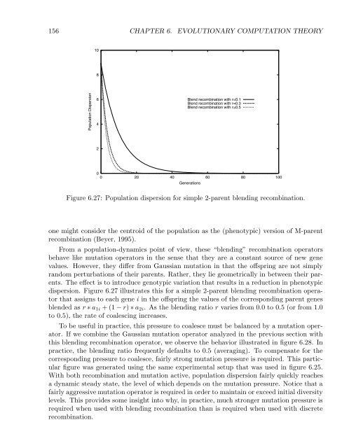
Figure 6.27: Population dispersion for simple 2-parent blending recombination.
one might consider the centroid of the population as the (phenotypic) version of M-parent
recombination (Beyer, 1995).
From a population-dynamics point of view, these “blending” recombination operators
behave like mutation operators in the sense that they are a constant source of new gene
values. However, they differ from Gaussian mutation in that the offspring are not simply
random perturbations of their parents. Rather, they lie geometrically in between their parents.
The effect is to introduce genotypic variation that results in a reduction in phenotypic
dispersion. Figure 6.27 illustrates this for a simple 2-parent blending recombination operator
that assigns to each gene i in the offspring the values of the corresponding parent genes
blended as r ∗ a 1i +(1− r) ∗ a 2i . As the blending ratio r varies from 0.0 to 0.5 (or from 1.0
to 0.5), the rate of coalescing increases.
To be useful in practice, this pressure to coalesce must be balanced by a mutation operator.
If we combine the Gaussian mutation operator analyzed in the previous section with
this blending recombination operator, we observe the behavior illustrated in figure 6.28. In
practice, the blending ratio frequently defaults to 0.5 (averaging). To compensate for the
corresponding pressure to coalesce, fairly strong mutation pressure is required. This particular
figure was generated using the same experimental setup that was used in figure 6.25.
With both recombination and mutation active, population dispersion fairly quickly reaches
a dynamic steady state, the level of which depends on the mutation pressure. Notice that a
fairly aggressive mutation operator is required in order to maintain or exceed initial diversity
levels. This provides some insight into why, in practice, much stronger mutation pressure is
required when used with blending recombination than is required when used with discrete
recombination.