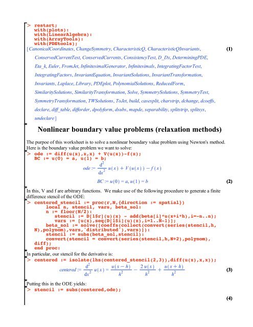
Nonlinear boundary value problems (relaxation methods)

O restart;
with(plots):
with(LinearAlgebra):
with(ArrayTools):
with(PDEtools);
CanonicalCoordinates, ChangeSymmetry, CharacteristicQ, CharacteristicQInvariants,
ConservedCurrentTest, ConservedCurrents, ConsistencyTest, D_Dx, DeterminingPDE,
Eta_k, Euler, FromJet, InfinitesimalGenerator, Infinitesimals, IntegratingFactorTest,
IntegratingFactors, InvariantEquation, InvariantSolutions, InvariantTransformation,
Invariants, Laplace, Library, PDEplot, PolynomialSolutions, ReducedForm,
SimilaritySolutions, SimilarityTransformation, Solve, SymmetrySolutions, SymmetryTest,
SymmetryTransformation, TWSolutions, ToJet, build, casesplit, charstrip, dchange, dcoeffs,
declare, diff_table, difforder, dpolyform, dsubs, mapde, separability, splitstrip, splitsys,
undeclare
Nonlinear boundary value problems (relaxation methods)
(1)
The purpoe of this worksheet is to solve a nonlinear boundary value problem using Newton's method.
Here is the boundary value problem we want to solve:
O ode := diff(u(x),x,x) + V(u(x))-f(x);
BC := u(0) = a, u(1) = b;
ode :=
d2
dx 2 u x C V u x K f x
BC := u 0 = a, u 1 = b
(2)
In this, V and f are arbitrary functions. We make use of the following procedure to generate a finite
difference stencil of the ODE:
O centered_stencil := proc(r,N,{direction := spatial})
local n, stencil, vars, beta_sol:
n := floor(N/2):
stencil := D[1$r](u)(x) - add(beta[i]*u(x+i*h),i=-n..n);
vars := [u(x),seq(D[1$i](u)(x),i=1..N-1)];
beta_sol := solve([coeffs(collect(convert(series(stencil,h,
N),polynom),vars,'distributed'),vars)]):
stencil := subs(beta_sol,stencil):
convert(stencil = convert(series(stencil,h,N+2),polynom),
diff);
end proc:
In particular, our stencil for the derivative is:
O centered := isolate(lhs(centered_stencil(2,3)),diff(u(x),x,x));
centered :=
d2
dx 2 u x = u x K h
h 2 K 2 u x
h 2 C u x C h
h 2
Putting this in the ODE yields:
O stencil := subs(centered,ode);
(3)
(4)

stencil := u x K h
h 2
K 2 u x
h 2
C u x C h
h 2 C V u x K f x
(4)
We relabel various things for ease of reading:
O Subs1 := [seq(u(x+i*h)=u[j+i],i=-1..1),f(x)=f[j]];
Subs1 := u x K h = u j K 1
, u x = u j
, u x C h = u j C 1
, f x = f j
In terms of these, the stencil becomes
O stencil := expand(subs(Subs1,stencil)*(-h^2/2));
stencil := K 1 2 u j K 1 C u j K 1 2 u j C 1 K 1 2 h2 V u j
C 1 2 h2 f j
Now, if V is a nonlinear function, this will be a set of nonlinear equations for u[j]. We linearize the
equations the equations by first make the substitutions:
O Subs2 := [seq(u[j+i]=U[j+i]+epsilon*dU[j+i],i=-1..1)];
Subs2 := u j K 1
= U j K 1
C e dU j K 1
, u j
= U j
C e dU j
, u j C 1
= U j C 1
C e dU j C 1
(5)
(6)
(7)
In this, U is a guess for u and dU is the error in that guess. Putting these into stencil and then expanding
to linear order in epsilon yields:
O linear_stencil := series(subs(Subs2,stencil),epsilon,2);
linear_stencil := convert(linear_stencil,polynom);
linear_stencil := collect(subs(epsilon=1,(linear_stencil = 0)-
subs(epsilon=0,linear_stencil)),[dU[j-1],dU[j],dU[j+1]]);
linear_stencil := K 1 2 U j K 1 C 1 2 h2 f j
C U j
K 1 2 U j C 1 K 1 2 h2 V U j
C dU j
K 1 2 dU j K 1 K 1 2 h2 D V U j
dU j
K 1 2 dU j C 1
e C O e 2
linear_stencil := K 1 2 U j K 1 C 1 2 h2 f j
C U j
K 1 2 U j C 1 K 1 2 h2 V U j
C dU j
K 1 2 dU j K 1 K 1 2 h2 D V U j
dU j
K 1 2 dU j C 1
e
linear_stencil := K 1 2 dU j K 1 C 1 K 1 2 h2 D V U j
dU j
K 1 2 dU j C 1 = 1 2 U j K 1
(8)
K 1 2 h2 f j
K U j
C 1 2 U j C 1 C 1 2 h2 V U j
Written in this way, we see that linear stencil is a tridiagonal matrix problem for the error vector dU. The
procedure GenerateSystem take an initial guess U, and the various quantites appearing in the ODE (a b,
V, f) and a stepsize h and returns the linear system to be solve for dU in matrix form.
O beta := unapply(rhs(linear_stencil),j,U,h,V,f); # This procedure
generates the RHS of linear stencil for each j
GenerateSystem := proc(U,a,b,V,f,h)
local M, UU, A, B:
M := Dimension(U):
UU := Array(0..M+1,[a,op(convert(U,list)),b]): # We augment
the initial guess for the solution vector by adding the BCs at
either end

A := BandMatrix([[-1/2$(M-1)],[seq(1-1/2*h^2*D(V)(UU[i]),i=1.
.M)],[-1/2$(M-1)]],1,M): # this matrix reproduces the LHS of
linear stencil
B := Vector(1..M,[seq(beta(i,UU,h,V,f),i=1..M)]); # This
vector is the RHS of linear stencil for all j
A,B:
end proc:
b :=
j, U, h, V, f / 1 2 U j K 1 K 1 2 h2 f j
K U j
C 1 2 U j C 1 C 1 2 h2 V U j
(9)
We test our GenerateSystem procedure on a dummy guess vector UU with five entries.
O M := 5;
UU := Vector([seq(U[i],i=1..M)]);
GenerateSystem(UU,a,b,V,f,h);
M := 5
U 1
U 2
UU :=
U 3
U 4
U 5
1 K 1 2 h2 D V U 1
, K 1 2
, 0, 0, 0 ,
(10)
K 1 2 , 1 K 1 2 h2 D V U 2
, K 1 2 , 0, 0 ,
0, K 1 2 , 1 K 1 2 h2 D V U 3
, K 1 2 , 0 ,
0, 0, K 1 2 , 1 K 1 2 h2 D V U 4
, K 1 2 ,
0, 0, 0, K 1 2 , 1 K 1 2 h2 D V U 5
,
1
2 a K 1 2 h2 f 1
K U 1
C 1 2 U 2 C 1 2 h2 V U 1
1
2 U 1 K 1 2 h2 f 2
K U 2
C 1 2 U 3 C 1 2 h2 V U 2
1
2 U 2 K 1 2 h2 f 3
K U 3
C 1 2 U 4 C 1 2 h2 V U 3
1
2 U 3 K 1 2 h2 f 4
K U 4
C 1 2 U 5 C 1 2 h2 V U 4
1
2 U 4 K 1 2 h2 f 5
K U 5
C 1 2 b C 1 2 h2 V U 5

Notice how a and b (the parameters in the boundary condition) appear in the B vector. The algoirthm we
pursue is similar to the one employed for the nonlinear Crank-Nicholson problem: We guess the solution
vector U, solve the linear system from GenerateSystem for dU, and then update our original guess via U
= U + dU. The algoirthm terminates when dU gets small; i.e., with the RMS value of each component in
dU is less than a tolerance eps. BVP_solver is an implementation of this algorithm:
O BVP_solver := proc(V,ff,a,b,M)
local h, x, f, U, p, CONTINUE, eps, i, gnat, dU, err:
h := evalf(1/(M+1)): # the stepsize
x := Array(0..M+1,[seq(h*i,i=0..M+1)]):
# an array containing x values of the lattice
f := map(x->ff(x),x):
# the array containing the f[j]'s in linear stencil
U := Vector(1..M,[seq(a+i/(M+1)*(b-a),i=1..M)],datatype=
float): # our initial guess (straight line between [0,a] and [1,
b]
p[0] := plot([[0,a],seq([x[i],U[i]],i=1..M),[1,b]],axes=
boxed,title=`iteration no. 0`): # first frame of a movie
CONTINUE := true:
eps := 1e-6: # the tolerance parameter that controls when
Newton iterations stop
for i from 1 to 50 while (CONTINUE) do:
gnat := GenerateSystem(U,a,b,V,f,h):
dU := LinearSolve(gnat): #
solving for dU
err := sqrt(dU.dU/M):
# err is
the RMS value of each component of dU
if (err < eps) then CONTINUE := false fi: # if err
< eps the loop stops
U := U + dU: # updating the value of U
p[i] := plot([[0,a],seq([x[j],U[j]],j=1..M),[1,b]],
axes=boxed,title=cat(`iteration no. `,i)): # next movie frame
od:
display(convert(p,list),insequence=true):
# the
output is a movie of each stage of the Newton iterations
end proc:
The output of BVP_solver is a movie of the shape of our numeric solution of the BVP after each Newton
iteration. Here is an example of the output for a nonlinear and inhomogeneous problem:
O ff := x -> 5/(1+x^2):
VV := u -> u*(1-u):
aa := 20:
bb := 25:
BVP := [collect(dsubs(V=VV,f=ff,ode),[diff(u(x),x,x),u(x)],
factor),op(dsubs(a=aa,b=bb,{BC}))];
movie := BVP_solver(VV,ff,aa,bb,100):
movie;
d 2
BVP :=
dx 2 u x K u x 2 C u x K 5 , u 0 = 20, u 1 = 25
2
1 C x

25
iteration no. 0
20
15
10
0 0.2 0.4 0.6 0.8 1
One can also get dsolve/numeric to solve the BVP for comparison
O UU := rhs(dsolve(BVP,numeric,output=listprocedure)[2]);
still := plot(UU(x),x=0..1,color=blue,axes=boxed):
still;
UU := proc x ... end proc

25
20
15
10
0 0.2 0.4 0.6 0.8 1
x
Here is the movie and the still diplayed together. One can see it only take a few iterations for our method
(red) to closely match the output of dsolve/numeric (blue).
O display([movie,still]);

25
iteration no. 5
20
15
10
0 0.2 0.4 0.6 0.8 1
x