Autumn 2003.

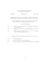
Department of Mathematics & Statistics
Stat 2593 Final Examination
13 December 2003
TIME: 3 hours. Total Marks: 75.
You are permitted to use one 8 & 1/2 × 11 “crib sheet” of notes and formulae
in this exam, and a calculator. Any statistical tables that you may need are
amongst those that are attached at the back of the question paper.
Indicate your answers clearly. Show all work.
1. Shipments of drive shafts arrive intermittently at a distribution warehouse. In each
shipment there is a (random) number of used drive shafts; the rest are new. Let X
be the number of used drive shafts in a randomly selected shipment.
Suppose that the probability mass function for X is as given in the following table:
x 0 1 2 3 4 5 6
P (X = x) 0.04 0.13 0.29 0.20 0.13 0.06
(a) What is the probability that X = 1 1 mark
(b) Calculate P (X = 5 | X ≥ 3). (Give your answer to FOUR decimal places.) 2 marks
(c) Are the events “X = 5” and X ≥ 3 mutually exclusive Explain briefly. 1 mark
(d) Are the events “X = 5” and X ≥ 3 independent Explain briefly. 1 mark
2. Let X be a random variable with probability density function 4 marks
f(x) = 3x2
875
for 5 ≤ x ≤ 10
(f(x) = 0 elsewhere).
Let h(X) = 1/(1 + X 3 ). Find the expected value of the random variable h(X). (Give
your answer to FOUR decimal places.)
3. Laxmark Printers buys a shipment of toner cartridges from The Great Australian
Blott Proprietary Ltd. Because of the “Near enough is good enough, she’ll be right,
mate” Australian attitude, 20% of the cartridges produced by the Blott Proprietary
are defective in some way.
(a) Suppose that Laxmark buys 8 of these cartridges. What is the probability that 3 marks
at least 2 of them are defective
(b) Suppose that Laxmark buys 80 of these cartridges. What is the probability that 3 marks
at least 20 of them are defective

4. The following is a stem-leaf plot of the farkling fraction (in furlongs per fortnight) of
a random sample of Lesser Tasmanian Drop-Bears:
MTB > stem c1
Stem-and-leaf of far.frac N = 75
Leaf Unit = 0.10
4 0 2558
12 1 00567899
21 2 011223357
29 3 00136669
(13) 4 0012233566778
33 5 1458
29 6 22459
24 7 446789
18 8 04558
13 9 3
12 10 24468
7 11 1
6 12
6 13 3
5 14
5 15 2468
1 16
1 17 3
(a) Comment briefly on the shape of the distribution of these data. 1 mark
(b) Would it be reasonable to assume that the population of farkling fractions of all 1 mark
Lesser Tasmanian Drop Bears has a normal (Gaussian) distribution Explain
briefly.
(c) Determine the median of this sample. 1 mark
(d) Will the mean of these data be larger or smaller than the median Explain 1 mark
briefly.
(e) The “hinges” (roughly the same as the 1st and 3rd quartiles) of this data set are 1 mark
2.4 and 7.85. What is the very longest that the whiskers of a boxplot of these
data could be
(f) What is the tip (right hand endpoint) of the right hand whisker of a boxplot of 1 mark
these data
(g) What is the tip (left hand endpoint) of the left hand whisker of a boxplot of 1 mark
these data
(h) Are there (according to the boxplot criterion) any outliers in this data set If 1 mark
so, what are their values
2

5. Tensile strength tests were carried out on two different grades (“AISI 1064” and “AISI
1078”) of wire rod. The resulting data were entered into a Minitab worksheet. Given
below is the output of two Minitab analyses of these data. One of the analyses is
CORRECT; the other is SILLY.
MTB > # Analysis number 1.
MTB > TwoSample ’AISI1078’ ’AISI1064’
Two-sample T for AISI1078 vs AISI1064
N Mean StDev SE Mean
AISI1078 129 123.60 2.00 0.18
AISI1064 129 107.60 1.30 0.11
Difference = mu AISI1078 - mu AISI1064
Estimate for difference: 16.000
95% CI for difference: (15.586, 16.414)
T-Test of difference = 0 (vs not =): T-Value = 76.18 P-Value = 0.000 DF = 219
===+===+===+===+===+===+===+===+===+===+===+===+===+===+===+===+===+===+===
MTB > # Analysis number 2.
MTB > let c3 = c1 - c2
MTB > name c3 ’Hi - Lo’
MTB > OneT ’Hi - Lo’
Variable N Mean StDev SE Mean 95.0% CI
Hi - Lo 129 16.000 2.373 0.209 ( 15.587, 16.413)
(a) State which is the correct analysis, explaining why briefly. 2 marks
(b) Using the correct analysis, specify a 95% confidence interval for the population 1 mark
mean difference in tensile strength between the higher grade (AISI 1078) and
lower grade (AISI 1064) wire rods. (Give your answer to THREE decimal
places.)
(c) Should you believe the assertion that on average the higher grade rods exceed 2 marks
the lower grade rods in tensile strength by 10 kg/mm 2 Explain briefly.
NOTE: You will receive ZERO marks for an answer based on the wrong analysis.
6. In a sample of 120 half-inch steel anchor bolts, 102 had shear strength less than or 4 marks
equal to 9.0 kip. Estimate at the 90% confidence level the proportion of all half-inch
steel anchor bolts having shear strength less than or equal to 9.0 kip.
3

7. The unrestrained compressive strength of a particular type of brick has a gamma
distribution with mean equal to 3000 psi and standard deviation equal to 1200 psi. It
is desired to find the probability that the compressive strength is at least 2000 psi.
(a) Find the parameters α and β of the gamma distribution in question. 3 marks
(b) The following Minitab output displays three calculations, one of which is relevant 2 marks
to answering the question of interest, and two of which are SILLY. Making use of
the appropriate portion of the output, find the probability that the unrestrained
compressive strength of a randomly selected brick of the given type is at least
2000 psi. Note: In this Minitab output, k1 and k2 are Minitab constants which
have been assigned the correct values of α and β respectively.
MTB > # First calculation which involved clicking on
MTB > # Probability density. Input constant equal to 2000.
MTB > PDF 2000;
SUBC> Gamma k1 k2.
Probability Density Function
Gamma with a = ******* and b = *******
x f( x )
2.00E+03 0.0003
===+===+===+===+===+===+===+===+===+===+===+===+===+===+===+===+===+===+===
MTB > # Second calculation which involved clicking on cumulative
MTB > # probability. Input constant equal to 2000.
MTB > CDF 2000;
SUBC> Gamma k1 k2.
Cumulative Distribution Function
Gamma with a = ******* and b = *******
x P( X # Third calculation which involved clicking on inverse
MTB > # cumulative probability. Input constant equal to 0.6667.
MTB > InvCDF 0.6667;
SUBC> Gamma k1 k2.
Inverse Cumulative Distribution Function
Gamma with a = ******* and b = *******
P( X

8. A random sample of individuals who drive alone to work in a large metropolitan area
was obtained. Each individual was categorized with respect to size of car driven and
with respect to commuting distance. The resulting table was analyzed in Minitab; the
results (parts of which have been obliterated) are shown below. Row 1 of the table
corresponds to “subcompact”, row 2 to “compact”, row 3 to “midsize” and row 4 to
“full-size”. The column names classify the commuting distance (in kilometres).
MTB > chis c1-c3
Expected counts are printed below observed counts
0-

(b) A plant producing electronic components has samples of 200 components selected 4 marks
daily from its output. The number of non-conforming components is determined,
and the corresponding sample proportion is plotted on a control chart having a
centre line of p = 0.15, an upper control limit UCL = 0.2257, and and a lower
control limit LCL = 0.0743.
Suppose that events take place which cause the proportion of non-conforming
components in the plant’s product to change from 0.15 to 0.10. What is the
probability that a single sample (of 200 components) taken after the change, will
provide evidence that the change has occurred
10. Hexavalent chromium is a carcinogenic air toxin of substantial concern. In a study
on the prevalence of this toxin data were collected on the indoor and outdoor concentrations
(in ng/m 3 ) of hexavalent chromium, at a number of randomly selected
houses in a region of Southern Ontario. One of the objectives of the study was to
demonstrate that, on average, the outdoor concentrations were higher than the indoor
ones. The resulting data were entered into a Minitab worksheet. Given below is the
output (parts of which have been obliterated) of two Minitab analyses of these data.
One of the analyses is CORRECT; the other is SILLY.
MTB > # Analysis number 1:
MTB > TwoSample ’Outdoor’ ’Indoor’;
SUBC> Alternative **.
N Mean StDev SE Mean
Outdoor 33 0.637 0.392 0.068
Indoor 33 0.231 0.128 0.022
Difference = mu Outdoor - mu Indoor
Estimate for difference: 0.4061
*** (Line omitted) ***
T-Test of difference = 0 (vs **): T-Value = 5.65 P-Value = 0.000 DF = 38
MTB > # Analysis number 2:
MTB > let c3 = c1 - c2
MTB > name c3 ’O - I’
MTB > OneT ’O - I’;
SUBC> Test 0;
SUBC> Alternative **.
Test of mu = 0 vs mu ****
Variable N Mean StDev SE Mean
O - I 33 0.4061 0.3920 0.0682
Variable ***************** T P
O - I ***************** 5.95 0.000
. . . . . . (continued over page)
6

10. (Continued.)
(a) State which is the correct analysis, explaining why briefly. 2 marks
(b) On the basis of the (correct) Minitab analysis, state clearly your decision about 1 marks
the hypothesis being tested, at each of the “standard” significance levels, i.e.
0.10, 0.05, and 0.01.
(c) Explain briefly, in a way that a non-statistician could understand, what your 2 marks
decision means.
(d) There were 33 houses involved in the study; if a 34th house were to be ran- 3 marks
domly selected from the given region, between what values would you predict
the outdoor minus indoor difference in concentrations to lie
NOTE: You will receive ZERO marks for an answer based on the wrong analysis.
11. In biofiltration of wastewater, the ambient temperature is known to have a substantial
impact on the efficiency of filtration. In a study done on this subject, data were
collected on the inlet temperature (in degrees C.) and the removal efficiency in percent
for a particular biofiltration facility. A linear regression model to predict efficiency
from temperature was fitted to the resulting data set in Minitab. The resulting output,
parts of which have been obliterated, is shown below.
MTB > set c3
DATA> 9 10.5 14
DATA> end
MTB > regr c2 1 c1;
SUBC> pred c3.
The regression equation is
removal = 97.5 + 0.0757 temp
Predictor Coef SE Coef T P
Constant 97.4986 0.0889 1096.17 0.000
temp 0.075691 0.007046 10.74 0.000
S = 0.1552 R-Sq = 79.4% R-Sq(adj) = 78.7%
Analysis of Variance
Source DF SS MS F P
Regression 1 2.7786 2.7786 115.40 0.000
Residual Error 30 0.7224 0.0241
Total 31 3.5010
. . . . . . (continued over page)
7

11. (Continued.)
Predicted Values for New Observations
New Obs Fit SE Fit 95.0% CI 95.0% PI
1 98.1798 0.0347 ( 98.1090, 98.2506) ( 97.8551, 98.5045)
2 ******* 0.0294 ( *******, *******) ( *******, *******)
3 98.5583 0.0308 ( 98.4953, 98.6212) ( 98.2352, 98.8814)
Values of Predictors for New Observations
New Obs temp
1 9.0
2 10.5
3 14.0
(a) Clearly the inlet temperature must be above freezing for filtration to take place 1 . 4 marks
Suppose that it is claimed that when the temperature is “just marginally above
freezing” the removal efficiency is, on average, at most 97.2%. Check this claim,
on the basis of the available analysis, by testing an appropriate hypothesis. Explain
in one brief sentence your choice of alternative hypothesis. In terms of your
test, does the claim appear to be valid
(Hint: Ignore the fact that if the temperature is 0 ◦ then filtration cannot take place;
i.e. consider “just marginally above freezing” to be 0 ◦ . Then you are testing a
hypothesis about one simple parameter of the model. Which parameter)
(b) Find a 95% prediction interval for a single observation of efficiency when the 3 marks
temperature is 10.5 ◦ C.
(c) Suppose it is claimed that when the temperature is 14 ◦ C. the mean efficiency is 1 marks
98.6% Should you believe this claim Explain briefly.
(d) Suppose it is claimed that when the temperature is 9 ◦ C. the efficiency was 1 marks
observed to take a value of 98.6% Should you believe this claim Explain briefly.
12. Suppose that a 100 metre reel of magnetic tape of a certain type has 25 flaws, on
average.
(a) A 10 metre segment of such tape is selected at random. Under “reasonable” 2 marks
assumptions the number of flaws in this segment of tape has particular wellknown
distribution. Specify this distribution — i.e. give its name and state the
values of any associated parameters.
(b) Calculate (assuming this distribution) the probability that a 10 metre segment 2 marks
of such tape has exactly 2 flaws.
(c) Write down the probability density function for the distance in metres between 2 marks
successive flaws in such magnetic tape.
1 You can’t filter ice, mate!
8