Lecture 3: The Time Dependent Schrödinger Equation The ... - Cobalt
Lecture 3: The Time Dependent Schrödinger Equation The ... - Cobalt
Lecture 3: The Time Dependent Schrödinger Equation The ... - Cobalt

You also want an ePaper? Increase the reach of your titles
YUMPU automatically turns print PDFs into web optimized ePapers that Google loves.
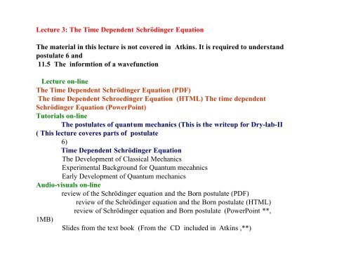
<strong>Lecture</strong> 3: <strong>The</strong> <strong>Time</strong> <strong>Dependent</strong> <strong>Schrödinger</strong> <strong>Equation</strong><br />
<strong>The</strong> material in this lecture is not covered in Atkins. It is required to understand<br />
postulate 6 and<br />
11.5 <strong>The</strong> informtion of a wavefunction<br />
<strong>Lecture</strong> on-line<br />
<strong>The</strong> <strong>Time</strong> <strong>Dependent</strong> <strong>Schrödinger</strong> <strong>Equation</strong> (PDF)<br />
<strong>The</strong> time <strong>Dependent</strong> Schroedinger <strong>Equation</strong> (HTML) <strong>The</strong> time dependent<br />
<strong>Schrödinger</strong> <strong>Equation</strong> (PowerPoint)<br />
Tutorials on-line<br />
<strong>The</strong> postulates of quantum mechanics (This is the writeup for Dry-lab-II<br />
( This lecture coveres parts of postulate<br />
6)<br />
<strong>Time</strong> <strong>Dependent</strong> <strong>Schrödinger</strong> <strong>Equation</strong><br />
<strong>The</strong> Development of Classical Mechanics<br />
Experimental Background for Quantum mecahnics<br />
Early Development of Quantum mechanics<br />
Audio-visuals on-line<br />
review of the <strong>Schrödinger</strong> equation and the Born postulate (PDF)<br />
review of the <strong>Schrödinger</strong> equation and the Born postulate (HTML)<br />
review of <strong>Schrödinger</strong> equation and Born postulate (PowerPoint **,<br />
1MB)<br />
Slides from the text book (From the CD included in Atkins ,**)
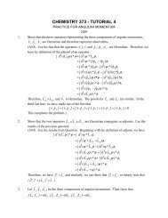
setting up equation<br />
Consider a particle of mass m that is moving in one<br />
dimension. Let its position be given by x<br />
V<br />
<strong>Time</strong> <strong>Dependent</strong> <strong>Schrödinger</strong> <strong>Equation</strong><br />
O<br />
V(X,t 1 ) V(X,t 2 )<br />
X<br />
Let the particle be<br />
subject to the<br />
potential V(x,t)<br />
O<br />
All properties of such a particle is in quantum mechanics<br />
determined by the wavefunction Ψ(x,t) of the system
<strong>Time</strong> <strong>Dependent</strong> <strong>Schrödinger</strong> <strong>Equation</strong><br />
Vxt ( , ) setting up equation<br />
X
<strong>Time</strong> <strong>Dependent</strong> <strong>Schrödinger</strong> <strong>Equation</strong><br />
setting up equation<br />
A system that changes with time<br />
is described by the time -<br />
dependent <strong>Schrödinger</strong> equation<br />
h δΨ( xt , )<br />
− =<br />
i δt<br />
Hˆ Ψ( x, t)<br />
Where Hˆ<br />
is the Hamiltonian of<br />
the system :<br />
Hˆ h 2 δ<br />
2 = − + Vxt ( , )<br />
2m δx<br />
2<br />
for<br />
1D - particle<br />
according to postulate 6
<strong>Time</strong> <strong>Dependent</strong> <strong>Schrödinger</strong> <strong>Equation</strong><br />
setting up equation<br />
2 2<br />
− hδΨ( xt , ) = − h δ Ψ( xt , )<br />
i δt<br />
2m<br />
2<br />
+<br />
δx<br />
Vxt ( , ) Ψ( xt , )<br />
<strong>The</strong> time dependent <strong>Schrödinger</strong> equation<br />
<strong>The</strong> wavefunction Ψ(x,t) is also referred to as<br />
<strong>The</strong> statefunction<br />
Our state will in general change with time due to V(x,t).<br />
Thus Ψ is a function of time and space
<strong>Time</strong> <strong>Dependent</strong> <strong>Schrödinger</strong> <strong>Equation</strong><br />
Probability from wavefunction<br />
<strong>The</strong> wavefunction does not have any physical interpretation.<br />
However :<br />
*<br />
P(x,t) = Ψ(x,t)<br />
Ψ(x,t) dx<br />
Probability density<br />
Is the probability at time t to find the particle<br />
between x and x + ∆x.<br />
Ψ( x,t)Ψ * ( x,t)dx<br />
will change with time<br />
dx<br />
o<br />
x
<strong>Time</strong> <strong>Dependent</strong> <strong>Schrödinger</strong> <strong>Equation</strong><br />
Probability from wavefunction<br />
It is important to note that the particle is not distributed<br />
over a large region as a charge cloud<br />
Ψ(x,t) Ψ(x,t) *<br />
It is the probability patterns (wave function) used<br />
to describe the electron motion that behaves like<br />
waves and satisfies a wave equation
<strong>Time</strong> <strong>Dependent</strong> <strong>Schrödinger</strong> <strong>Equation</strong><br />
Probability from wavefunction<br />
Consider a large number N of<br />
identical boxes with identical<br />
particles all described by the<br />
same wavefunction Ψ( xt , ):<br />
Let dn x denote the number of particle<br />
which at the same time is found<br />
between x and x + ∆x<br />
<strong>The</strong>n :<br />
dn x *<br />
=Ψ( xt , ) Ψ ( xtdx , )<br />
N
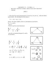
<strong>Time</strong> <strong>Dependent</strong> <strong>Schrödinger</strong> <strong>Equation</strong><br />
with time independent potential energy<br />
<strong>The</strong> time - dependent Schroedinger equation :<br />
2 2<br />
− hδΨ( xt , ) =− h δ Ψ( xt , )<br />
i δt<br />
2m<br />
2<br />
δx<br />
+<br />
Can be simplified<br />
in those cases where<br />
the potential V only<br />
depends on the<br />
position : V(t,x) - ><br />
V(x)<br />
V<br />
V(X)<br />
O<br />
Vxt ( , ) Ψ( xt , )
<strong>Time</strong> <strong>Dependent</strong> <strong>Schrödinger</strong> <strong>Equation</strong><br />
with time independent potential energy :<br />
separation of time and space<br />
We might try to find a solution of the form :<br />
Ψ( xt , ) = ft ( ) ψ( x)<br />
We have<br />
δΨ(x,t)<br />
δψ(<br />
(x)f(t))<br />
= = ψ(<br />
x) δf(t)<br />
δt δt δt<br />
δ<br />
and<br />
2<br />
2<br />
Ψ(x,t) δψ( (x)f(t)) δψ(<br />
x)<br />
= = f(t)<br />
2<br />
2<br />
2<br />
δx δx δx<br />
2
Simplyfied <strong>Time</strong> <strong>Dependent</strong> <strong>Schrödinger</strong> <strong>Equation</strong><br />
with time independent potential energy :<br />
separation of time and space<br />
hδΨ( xt , ) h δ Ψ( xt , )<br />
− =− +<br />
i δt<br />
2m<br />
2<br />
δx<br />
A substitution of<br />
2 2<br />
Ψ( xt , ) = ft ( ) ψ( x)<br />
Vxt ( , ) Ψ( xt , )<br />
into the <strong>Schrödinger</strong> equation thus affords :<br />
2 2<br />
− h<br />
= − h<br />
ψ<br />
δ δψ(<br />
( x) f(t) x)<br />
f(t)<br />
2<br />
i δt 2m δx<br />
+<br />
Vx ( ) f(t) ψ(<br />
x)
Simplyfied <strong>Time</strong> <strong>Dependent</strong> <strong>Schrödinger</strong> <strong>Equation</strong><br />
with time independent potential energy :<br />
separation of time and space<br />
2 2<br />
h<br />
h<br />
− ψ<br />
δ δψ(<br />
( x) f(t) x)<br />
= − f(t) +<br />
2<br />
i δt 2m δx<br />
1<br />
A multiplication from the left by affords :<br />
f() t ψ( x)<br />
2 2<br />
h 1 δf(t)<br />
h 1 δψ(<br />
x)<br />
− = − +<br />
2<br />
if() t δt 2mψ(<br />
x) δx<br />
Vx ( ) f(t) ψ(<br />
x)<br />
Vx ( )<br />
<strong>The</strong> R.H.S. does not depend on t if we now assume that<br />
V is time independent. Thus, the L.H.S. must also be<br />
independent of t
Simplyfied <strong>Time</strong> <strong>Dependent</strong> <strong>Schrödinger</strong> <strong>Equation</strong><br />
with time independent potential energy :<br />
separation of time and space<br />
Thus :<br />
h 1 δf(t)<br />
− = E = constant<br />
ift () δt<br />
<strong>The</strong> L.H.S. does not depend on x so the R.H.S. must also<br />
be independent of x and equal to the same constant, E.<br />
h 2 1 δψ<br />
2 ( x)<br />
− + V( x) = E = constant<br />
2<br />
2m<br />
ψ(<br />
x) δx
We can now solve for f(t) :<br />
h 1 δf(t)<br />
− = E = constant<br />
ift () δt<br />
Or :<br />
Simplyfied <strong>Time</strong> <strong>Dependent</strong> <strong>Schrödinger</strong> <strong>Equation</strong><br />
with time independent potential energy :<br />
separation of time and space<br />
δf(t)<br />
i Et δ<br />
f() t<br />
=− h<br />
Now integrating from time t=0 to t=to on both sides affords:<br />
t<br />
o<br />
∫<br />
o<br />
δf(t)<br />
o<br />
i<br />
=−∫ Et δ<br />
f() t h<br />
t<br />
o
Simplyfied <strong>Time</strong> <strong>Dependent</strong> <strong>Schrödinger</strong> <strong>Equation</strong><br />
with time independent potential energy :<br />
separation of time and space<br />
t<br />
o<br />
∫<br />
o<br />
δf(t)<br />
o<br />
i<br />
=−∫ Et δ<br />
f() t h<br />
t<br />
o<br />
i<br />
ln[ ft ( o)] − ln[ fo ( )] = − Et [ o −0]<br />
h<br />
i<br />
ln[ f( to)] =− Et o + ln[ f ( o )]<br />
h<br />
Cons<br />
tan<br />
t<br />
ln[ f( t )]<br />
o<br />
i<br />
=− Et o +<br />
h<br />
C
Simplified <strong>Time</strong> <strong>Dependent</strong> <strong>Schrödinger</strong> <strong>Equation</strong><br />
with time independent potential energy :<br />
separation of time and space<br />
Or:<br />
ln[ f ( t i<br />
o)]<br />
=− Et o + C<br />
h<br />
i i<br />
f ()= t Exp<br />
⎡ − Et + C<br />
⎤ Exp C Exp Et<br />
⎣⎢ ⎦⎥ = [ ] ⎡ ⎣⎢<br />
− ⎤<br />
h<br />
h ⎦⎥<br />
E E<br />
f ( t ) = Exp[ C] ⎡ ⎤ (cos t isin t )<br />
⎣⎢ ⎦⎥ − ⎡ ⎤<br />
h ⎣⎢ h ⎦⎥
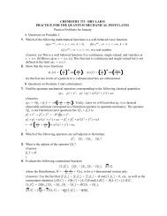
Simplified <strong>Time</strong> <strong>Dependent</strong> <strong>Schrödinger</strong> <strong>Equation</strong><br />
with time independent potential energy :<br />
separation of time and space<br />
E E<br />
f ( t ) = Exp[ C] ⎡ ⎤ (cos t isin t )<br />
⎣⎢ ⎦⎥ − ⎡ ⎤<br />
h ⎣⎢ h ⎦⎥<br />
+<br />
-<br />
i<br />
i<br />
- i +<br />
t = 0 t =π (h/ E) t = π(h/ E) t<br />
2 = 3π<br />
2 (h /E) t= 2π(h/ E)<br />
Change of<br />
sign of f(t)<br />
with time
Simplified <strong>Time</strong> <strong>Dependent</strong> <strong>Schrödinger</strong> <strong>Equation</strong><br />
with time independent potential energy :<br />
separation of time and space<br />
<strong>Time</strong> independent <strong>Schrödinger</strong> equation<br />
<strong>The</strong> equation for ψ(x) is given by<br />
h 2 1 δψ<br />
2 ( x)<br />
− + Vx ( ) =<br />
2m<br />
ψ(<br />
x)<br />
2<br />
δx<br />
E<br />
Or :<br />
h 2 2 2<br />
δψ(<br />
x)<br />
− + ψ( x) Vx ( ) = Eψ(<br />
x)<br />
2m δx
Simplified <strong>Time</strong> <strong>Dependent</strong> <strong>Schrödinger</strong> <strong>Equation</strong><br />
with time independent potential energy :<br />
separation of time and space<br />
<strong>Time</strong> independent <strong>Schrödinger</strong> equation<br />
h 2 2 2<br />
δψ(<br />
x)<br />
− + ψ( x) Vx ( ) = Eψ(<br />
x)<br />
2m δx<br />
This is the time-independent Schroedinger <strong>Equation</strong><br />
for a particle moving in the time independent potential V(x)<br />
It is a postulate of Quantum Mechanics that E is<br />
the total energy of the system<br />
Part of QM postulate 6
Simplified <strong>Time</strong> <strong>Dependent</strong> <strong>Schrödinger</strong> <strong>Equation</strong><br />
with time independent potential energy :<br />
separation of time and space<br />
<strong>Time</strong> independent <strong>Schrödinger</strong> equation<br />
<strong>The</strong> total wavefunction for a one-dimentional particle in<br />
a potential V(x) is given by<br />
Ψ( xt , ) = ft ( ) ψ( x)<br />
= Exp[ C] Exp[ −i E t] ψ( x)<br />
AExp[ i E h<br />
= − t] ψ( x)<br />
h
Simplified <strong>Time</strong> <strong>Dependent</strong> <strong>Schrödinger</strong> <strong>Equation</strong><br />
with time independent potential energy :<br />
separation of time and space<br />
<strong>Time</strong> independent <strong>Schrödinger</strong> equation<br />
If ψ(x) is a solution to<br />
h 2 2 2<br />
δψ(<br />
x)<br />
− + ψ( x) Vx ( ) = Eψ(<br />
x)<br />
2m δx<br />
So is A ψ(x)<br />
<strong>Lecture</strong> 2<br />
h 2 δ<br />
2 ( Aψ(<br />
x))<br />
− + Aψ( x) V( x) = AEψ(<br />
x)<br />
2<br />
2m δx
Simplified <strong>Time</strong> <strong>Dependent</strong> <strong>Schrödinger</strong> <strong>Equation</strong><br />
with time independent potential energy :<br />
separation of time and space<br />
time independent probability function<br />
h 2 δ<br />
2 ( Aψ(<br />
x))<br />
− + Aψ( x) V( x) = AEψ(<br />
x)<br />
2<br />
2m δx<br />
or :<br />
h 2 2 2<br />
δψ'(<br />
x)<br />
− + ψ'( x) Vx ( ) = Eψ'(<br />
x)<br />
2m δx<br />
with ψ<br />
' (x) = A ψ(x)
Simplified <strong>Time</strong> <strong>Dependent</strong> <strong>Schrödinger</strong> <strong>Equation</strong><br />
with time independent potential energy :<br />
separation of time and space<br />
time independent probability function<br />
Thus we can write without loss of generality for a<br />
particle in a time-independent potential<br />
Ψ( x, t) = Exp[ −i E t] ψ( x)<br />
h<br />
This wavefunction is time dependent and complex.<br />
Let us now look at the corresponding probability density<br />
Ψ( xt , ) Ψ<br />
*<br />
( xt , )
Simplified <strong>Time</strong> <strong>Dependent</strong> <strong>Schrödinger</strong> <strong>Equation</strong><br />
with time independent potential energy :<br />
separation of time and space<br />
time independent probability function<br />
We have :<br />
*<br />
Ψ( xt , ) Ψ ( xt , ) = Exp[ −i E t] ψ( x)<br />
h<br />
* *<br />
× Exp[ i E t] ψ ( x) = ψ( x) ψ ( x)<br />
h<br />
Thus , states describing systems with a time-independent<br />
potential V(x) have a time-independent (stationary)<br />
probability density.
Simplified <strong>Time</strong> <strong>Dependent</strong> <strong>Schrödinger</strong> <strong>Equation</strong><br />
stationary states<br />
*<br />
Ψ( xt , ) Ψ ( xt , ) = Exp[ −i E t] ψ( x)<br />
h<br />
* *<br />
× Exp[ i E t] ψ ( x) = ψ( x) ψ ( x)<br />
h<br />
This does not imply that the particle is stationary.<br />
However, it means that the probability of finding<br />
a particle in the interval x + -1/2∆x to x +1/2∆x is<br />
constant.
Simplified <strong>Time</strong> <strong>Dependent</strong> <strong>Schrödinger</strong> <strong>Equation</strong><br />
stationary states<br />
*<br />
ψ( x) ψ ( x)<br />
dx Independent of time<br />
We say that systems that can be described by<br />
wave functions of the type<br />
Ψ( x, t) = Exp[ −i E t] ψ( x)<br />
h<br />
Represent<br />
Stationary<br />
states
Simplified <strong>Time</strong> <strong>Dependent</strong> <strong>Schrödinger</strong> <strong>Equation</strong><br />
Postulate 6<br />
<strong>The</strong> time development of the<br />
state of an undisturbed system<br />
is given by the time - dependent<br />
<strong>Schrödinger</strong> equation<br />
h δΨ( xt , )<br />
− =<br />
i δt<br />
Hˆ Ψ( x, t)<br />
where H ˆ is the Hamiltonian<br />
(i.e. energy) operator<br />
for the quantum mechanical system
What you should know from this lecture<br />
1. You should know postulate 6 and the form of the<br />
time dependent <strong>Schrödinger</strong> equation<br />
h δΨ( xt , )<br />
− =<br />
i δt<br />
Hˆ Ψ( x, t)<br />
2. You should know that the wavefunction for<br />
systems where the potential energy is independent of<br />
time [V(x,t) → V(x)] is given by<br />
Ψ( x, t) = Exp[ −i E t] ( x)<br />
h<br />
ψ<br />
Where ψ( x)<br />
is a solution to the time - independent<br />
<strong>Schrödinger</strong> equation : Hψ( x) = Eψ(<br />
x),<br />
and E is the energy of the system.
What you should know from this lecture<br />
3. Systems with a time independent potential<br />
energy [V(x,t) → V(x) ] have a time - independent<br />
probability density :<br />
* *<br />
Ψ( xt , ) Ψ ( xt , ) = Exp[ −i E t] ψ( x) Exp[ i E t] ψ ( x)<br />
h<br />
h<br />
= ψ( x) ψ<br />
*<br />
( x).<br />
<strong>The</strong>y are called stationary states