Stochastic Pruning - Pixar Graphics Technologies
Stochastic Pruning - Pixar Graphics Technologies
Stochastic Pruning - Pixar Graphics Technologies

Create successful ePaper yourself
Turn your PDF publications into a flip-book with our unique Google optimized e-Paper software.
<strong>Stochastic</strong> <strong>Pruning</strong><br />
Robert L. Cook John Halstead<br />
<strong>Pixar</strong> Animation Studios<br />
Abstract<br />
Many renderers perform poorly on scenes that contain a lot of detailed<br />
geometry. Level-of-detail techniques can alleviate the load<br />
on the renderer by creating simplified representations of primitives<br />
that are small on the screen. Current methods work well when the<br />
detail is due to the complexity of the individual elements, but not<br />
when it is due to the large number of elements. In this paper, we introduce<br />
a technique for automatically simplifying this latter type of<br />
geometric complexity. Some elements are pruned (i.e., eliminated),<br />
and the remaining elements are altered to preserve the statistical<br />
properties of the scene.<br />
CR Categories: I.3.3 [Picture/Image generation]: Antialiasing—<br />
[I.3.7]: Three-Dimensional <strong>Graphics</strong> and Realism—Color, shading,<br />
shadowing, and texture<br />
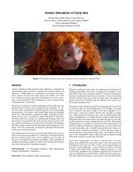
Figure 1: A plant with 320,000 leaves.<br />
Keywords: Level of detail, procedural models, Monte Carlo.<br />
1 Introduction<br />
Geometry can overwhelm a renderer. Highly detailed scenes can<br />
increase memory requirements and degrade performance, even to<br />
the point of becoming unrenderable. Fortunately, the amount of detail<br />
involved is typically too great to be represented at the resolution<br />
of the rendered image. In such cases, renderer performance can be<br />
greatly improved by substituting a less detailed version of the scene<br />
without perceptibly changing the image. Varying the level of detail<br />
processed by the renderer is crucial for efficient rendering of highly<br />
complex scenes.<br />
Creating these simplified representations manually [Crow 1982]<br />
can be prohibitively labor-intensive, so good automatic simplification<br />
techniques are important. Much of the research in this area has<br />
focused on simplifying complex surfaces (e.g., [Cohen et al. 1996]<br />
and [Lounsbery et al. 1997]), but these methods do not address one<br />
of the most important sources of geometric detail: complexity due<br />
to large numbers of simple, disconnected elements. For example,<br />
we recently had a landscape filled with plants like the one in Figure<br />
1 stretching from the near distance to the far horizon. The scene<br />
contained over a hundred million leaves and was unrenderable with<br />
RenderMan. Surface simplification techniques won’t help in this<br />
situation since the elements are already very simple.<br />
Some existing methods can simplify this type of complexity, but<br />
they have serious limitations. For some procedural models, the<br />
number of elements generated can be adjusted based on screen<br />
size (e.g., [Reeves 1983] and [Smith 1984]). This close coupling<br />
of level of detail with model generation tends to further complicate<br />
already intricate algorithms and does not help with expensive<br />
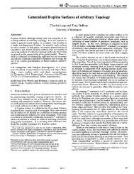
(a) (b) (c) (d)<br />
Figure 2: Distant views of the plant from Figure 1 with close-ups<br />
below: (a) unpruned, (b) with 90% of its leaves pruned, (c) with<br />
area correction, (d) with area and contrast correction.<br />
models that are pre-computed because they are expensive to generate<br />
(e.g., [Prusinkiewicz et al. 1994]). Image-based, 2-D approximations<br />
such as impostors and textured depth meshes are viewdependent<br />
(see [Wilson and Manocha 2003] for a good survey and<br />
analysis), and using 3-D volumetric representations (e.g., [Andujar<br />
et al. 2002]) can significantly degrade the appearance of the object.<br />
2 The Algorithm<br />
In this paper, we introduce stochastic pruning, a Monte Carlo technique<br />
for automatically simplifying objects made of a large number<br />
of geometric elements. When there are a large number of elements<br />
in a pixel, we estimate the color of the pixel from a subset of the elements.<br />
The unused elements are pruned, and the rest are altered to<br />
preserve the appearance of the object. The method is easy to implement<br />
and fit into a rendering pipeline, and it lets us render scenes of<br />
very high geometric complexity without sacrificing image quality.<br />
There are 4 guiding principles needed to make this approach work;<br />
we discuss each of these below.<br />
1. <strong>Pruning</strong> order. Deciding which elements to prune.<br />
2. Area preservation. Altering the size of the remaining elements<br />
so the total area of the object does not change.<br />
3. Contrast preservation. Altering the shading of the remaining<br />
elements so the contrast of image does not change.<br />
4. Smooth animation. Making pruned elements fade out instead<br />
of pop off.
Figure 3: u as a function of z at different pruning rates.<br />
(a)<br />
2.1 <strong>Pruning</strong> Order<br />
The farther away an object is, the smaller it is on the screen, the<br />
more elements there are per pixel, and the more we can prune. We<br />
need to determine u, the fraction of the elements that are unpruned,<br />
as a function of z, the distance from the camera. There are many<br />
ways this could be done. Since the number of elements per pixel is<br />
proportional to z −2 , we chose to use a similar formula for u:<br />
u = z −log h2<br />
where h is the distance at which half the elements are pruned; this<br />
controls how aggressively elements are pruned as they get smaller<br />
(see Figure 3). Note that for simplicity we have scaled z so that<br />
z = 1 where pruning begins; this should be where the shapes of<br />
individual elements are no longer discernible, usually when they<br />
are about the size of a pixel. As a result, this z scaling will depend<br />
on the image resolution.<br />
For animation, the elements must be pruned in a consistent order.<br />
This pruning order should not be correlated with geometric position,<br />
size, orientation, color, or other characteristics (e.g., pruning<br />
elements from left to right would be objectionable). Some objects<br />
are constructed in such a way that the pruning order can be determined<br />
procedurally, but we have found it more general and useful to<br />
determine the pruning order stochastically. A simple technique is to<br />
assign a random number to each element, then sort the elements by<br />
their random numbers. This is usually sufficient in practice, but using<br />
stratified sampling ([Cook 1986], [Mitchell 1987]) assures that<br />
elements close to each other geometrically are not close to each<br />
other in the pruning order. This spreads out the visual effects of<br />
pruning during animation and allows more aggressive pruning.<br />
When n, the number of elements in the object, is large, the time<br />
spent doing even trivial rejects can be significant, so we need for<br />
the pruned elements to not even be considered. This can be done<br />
by storing the elements in a file in reverse pruning order so that<br />
only the first nu elements in the file need to be read at rendering<br />
time. This file can be created as a post-process with any model.<br />
It works especially well in a film production environment, where<br />
the common case is to create sets from randomly scaled and rotated<br />
versions of a small number of pre-built plant shapes.<br />
2.2 Area preservation<br />
The total area of the object is na, where a is the average surface area<br />
of the individual elements. <strong>Pruning</strong> decreases the total area to nua;<br />
to compensate for this, the area of the unpruned elements should be<br />
scaled by an amount s unpruned so that:<br />
(1)<br />
(nu)(as unpruned ) = na (2)<br />
Therefore s unpruned = 1/u. Figure 4a shows the area scaling factor s<br />
as a function of x, the position of the element in the reverse pruning<br />
order. s is 1/u for unpruned elements (x < u) and 0 for pruned<br />
elements (x > u).<br />
(b)<br />
Figure 4: For smaller values of u, more elements are pruned (have<br />
0 area), and the remaining elements are enlarged more. In (a), elements<br />
are pruned abruptly; in (b) the pruning is gradual.<br />
For example, the unpruned plant in Figure 2a is noticeably less<br />
dense when 90% of its leaves have been pruned, as shown in Figure<br />
2b. In Figure 2c, we correct for this by making the remaining<br />
leaves 10 times larger so that the total area of the plant remains the<br />
same. Depending on the type of element, this can be done by scaling<br />
in one or two dimensions; in this example, the leaf widths are<br />
scaled, as shown in close-up view in Figure 2c. The widening visible<br />
in this magnified view is not noticeable in practice because the<br />
elements are so small their shapes are not discernible.<br />
2.3 Contrast preservation<br />
From the central limit theorem, we know that sampling more elements<br />
per pixel decreases the pixel variance. As a result, pruning<br />
an object (i.e., sampling fewer elements) increases its contrast (i.e.,<br />
higher variance). For example, notice how the pruned plant in Figure<br />
2c has a higher contrast than the unpruned plant in Figure 2a.<br />
We now analyze this effect and show how to compensate for it.<br />
The variance of the color of the elements is<br />
σ 2 elem = n<br />
∑<br />
i=1(c i − ¯c) 2 (3)<br />
where c i is the color of the i th element and ¯c is the mean color.<br />
When k elements are sampled per pixel, the expected variance of<br />
α<br />
σ 2<br />
a<br />
c<br />
h<br />
k<br />
n<br />
s<br />
t<br />
u<br />
x<br />
z<br />
amount of color variance reduction<br />
variance<br />
element surface area<br />
color<br />
z at which half the elements are pruned<br />
number of elements per pixel<br />
number of elements in the object<br />
area scaling correction factor<br />
size of transition region for fading out pruned elements<br />
fraction of elements unpruned<br />
position of an element in the reverse pruning order<br />
distance from the camera<br />
Figure 5: Some symbols used in this paper
Figure 6: Contrast correction is more important for aggressive pruning<br />
(small h). Parameters: k 1 = 1, k max = 121<br />
the pixels is related to the variance of the elements by:<br />
σ 2 pixel = k<br />
∑<br />
i=1(w i ) 2 σ 2 elem (4)<br />
where the weight w i is the amount the i th element contributes to<br />
the pixel. For this analysis, we can assume that each element contributes<br />
equally to the pixel with weight 1/k:<br />
σ 2 pixel = k<br />
∑<br />
i=1( 1 k )2 σ 2 elem = k( 1 k )2 σ 2 elem = 1 k σ 2 elem (5)<br />
The pixel variance when the unpruned object is rendered is:<br />
σ 2 unpruned = σ 2 elem /k unpruned (6)<br />
and the pixel variance when the pruned object is rendered is:<br />
σ 2 pruned = σ 2 elem /k pruned (7)<br />
We can make these the same by altering the colors of the pruned<br />
elements to bring them closer to the mean:<br />
c ′ i = ¯c + α(c i − ¯c) (8)<br />
which reduces the variance of the elements to:<br />
σ ′ 2<br />
elem =<br />
=<br />
n<br />
∑ (c ′ i − ¯c) 2 (9)<br />
i=1<br />
n<br />
∑ ( ¯c + α(c i − ¯c) − ¯c) 2 (10)<br />
i=1<br />
= α 2 ∑<br />
n (c i − ¯c) 2 (11)<br />
i=1<br />
= α 2 σ 2 elem (12)<br />
which in turn reduces the variance of the pixels to:<br />
σ ′ 2<br />
pruned = σ ′ 2<br />
elem /k pruned (13)<br />
= σ 2 elem α2 /k pruned (14)<br />
= σ 2 unpruned α2 k unpruned /k pruned (15)<br />
We want σ ′ 2<br />
pruned = σunpruned 2 , which is true when<br />
α 2 = k pruned /k unpruned (16)<br />
An image of a pruned object with these altered element colors will<br />
then have the same variance as an image of the unpruned object<br />
with the original element colors.<br />
Because screen size varies as 1/z 2 , we would expect k unpruned =<br />
k 1 z 2 , where k 1 is the value of k at z = 1, which we can estimate<br />
by dividing n by the number of pixels covered by the object when<br />
z = 1. Similarly, we would expect k pruned = uk unpruned = uk 1 z 2 , so<br />
that α 2 = u. Many renderers, however, have a maximum number of<br />
visible objects per pixel k max (e.g., 64 if the renderer point-samples<br />
8x8 locations per pixel), and this complicates the formula for α:<br />
α 2 = min(uk 1z 2 ,k max )<br />
min(k 1 z 2 ,k max )<br />
(17)<br />
Figure 7: Ratio of rendering time and memory use with and without<br />
pruning as a function of distance for the animation in the supplementary<br />
material of the plant in Figure 1 receding into the distance.<br />
Figure 6 shows α as a function of z for values of h. Notice that the<br />
contrast only changes in the middle distance. When the object is<br />
close, the contrast is unchanged because there is no pruning. When<br />
the object is far away, the contrast is unchanged because there are<br />
more than k max unpruned elements per pixel, so that k max elements<br />
contribute to the pixel in both the pruned and unpruned cases. The<br />
maximum contrast difference occurs at z = √ k max /k 1 . The smaller<br />
u is at this distance, the larger this maximum will be; contrast correction<br />
is thus more important with more aggressive pruning (Figure<br />
6). Figure 2d shows the plant in Figure 2c with contrast correction.<br />
If there are different types of elements in a scene (e.g. leaves and<br />
grass), each type needs its own independent contrast correction. ¯c<br />
should be based on the final shaded colors of the elements, but it<br />
can be approximated by reducing the variance of the shader inputs.<br />
2.4 Smooth Animation<br />
As elements are pruned during an animation, they should gradually<br />
fade out instead of just abruptly popping off. This can be done by<br />
gradually making the elements either more transparent or smaller as<br />
they are pruned. The later is shown in Figure 4b, where the size t of<br />
the transition region is 0.1. The orange line shows that for a desired<br />
pruning level of 70% (u = .3), the first 20% of the elements in the<br />
reverse pruning order (x u+t = .4) are completely pruned. From x=.2<br />
to x=.4, the areas gradually decrease to 0. As we zoom in and u<br />
increases, the elements at x = .4 are gradually enlarged, reaching<br />
their fully-enlarged size when u = .5 (the yellow line). The area<br />
under each line is the total pruned surface area and is constant.<br />
3 Results and Conclusions<br />
Figure 7 shows memory usage and rendering time for the plant in<br />
Figure 1 as it recedes into the distance (see movie in supplementary<br />
material). Figure 8 shows a variety of plants rendered with this<br />
Figure 8: A gallery of different pruned objects.
Figure 9: A scene renderered with pruning that was unrenderable in RenderMan without pruning.<br />
technique. The scene in Figure 9 contains over one hundred million<br />
leaves and requires so much memory that without pruning it is<br />
unrenderable with RenderMan.<br />
<strong>Stochastic</strong> pruning is an automatic, straightforward level-of-detail<br />
method that can greatly reduce the geometric complexity of objects<br />
with large numbers of simple, disconnected elements. This type of<br />
complexity is not effectively addressed by previous methods. The<br />
technique fits well into a rendering pipeline, needing no knowledge<br />
of how the geometry was generated. It is also easy to implement:<br />
just randomly shuffle the elements into a file and use code like that<br />
in the Appendix to read just the unpruned elements. We have successfully<br />
used this technique in a production environment with a<br />
variety of models to render highly complex scenes that we found<br />
impossible to render otherwise.<br />
4 Acknowledgments<br />
Omitted for anonymous review.<br />
References<br />
ANDUJAR, C., BRUNET, P., AND AYALA, D. 2002. Topologyreducing<br />
surface simplifications using a discrete solid representation.<br />
ACM Transaction on <strong>Graphics</strong> 21, 2 (April), 88–105.<br />
COHEN, J., VARSHNEY, A., MANOCHA, D., TURK, G., WE-<br />
BER, H., AGARWAL, P., BROOKS, F., AND WRIGHT, W. 1996.<br />
Simplification envelopes. In SIGGRAPH ’96 Proceedings, ACM<br />
Press, New York, NY, 119–128.<br />
COOK, R. 1986. <strong>Stochastic</strong> sampling in computer graphics. ACM<br />
Transaction on <strong>Graphics</strong> 5, 1 (January), 51–72.<br />
CROW, F. C. 1982. A more flexible image generation environment.<br />
In SIGGRAPH ’82 Proceedings, 9–18.<br />
LOUNSBERY, M., DEROSE, T., AND WARREN, J. 1997. Multiresolution<br />
analysis for surfaces of arbitrary topological type. ACM<br />
Transaction on <strong>Graphics</strong> 16, 1 (January), 34–73.<br />
MITCHELL, D. 1987. Generating antialiased images at low sampling<br />
densities. In SIGGRAPH ’87 Proceedings, 65–72.<br />
PRUSINKIEWICZ, P., JAMES, M., AND MECH, R. 1994. Synthetic<br />
topiary. In SIGGRAPH ’94 Proceedings, 351–358.<br />
REEVES, B. 1983. Particle systems - a technique for modeling<br />
a class of fuzzy objects. ACM Transaction on <strong>Graphics</strong> 2, 2<br />
(April), 91–108.<br />
SMITH, A. 1984. Plants, fractals, and formal languages. In SIG-<br />
GRAPH ’84 Proceedings, 1–10.<br />
WILSON, A., AND MANOCHA, D. 2003. Simplifying complex<br />
environments using incremental textured depth meshes. In SIG-<br />
GRAPH ’03 Proceedings, 678–688.<br />
Appendix. Sample code<br />
// This code was written as a compact example, not for speed or generality.<br />
// For example, these are in-memory routines, but in practice the elements<br />
// would be streamed in from a file.<br />
// The "Prune" routine takes an array "eIn" of elements in reverse pruning order<br />
// at distance "z", and returns a pruned array of elements "eOut" to be rendered.<br />
// These graphs illustrate how s and t change near u=0 and u=1:<br />
//<br />
// (when u-trans1)<br />
// sMax-> s ...sss