Classical and Improved Diffusion Theory for Subsurface Scattering

Classical and Improved Diffusion Theory
for Subsurface Scattering
Ralf Habel 1 Per H. Christensen 2 Wojciech Jarosz 1
1 Disney Research Zürich 2 Pixar Animation Studios
Technical report, June 2013
Abstract
This technical report provides a description and comparison of classical and improved diffusion theory as used for
rendering subsurface scattering in computer graphics. We discuss the searchlight problem and describe the diffusion
equation and Green’s functions of each diffusion theory. We discuss the commonly used single-depth approximation
leading to the diffusion dipole and elaborate on its connection to the desired extended-source function.
1. Introduction
This technical report provides an overview of classical and
improved diffusion theory as introduced in physics and related
fields, and utilized for rendering subsurface scattering
in computer graphics.
When introducing the quantized diffusion method for subsurface
scattering, d’Eon and Irving [dI11] presented several
improvements to diffusion theory in tandem with their proposed
solution (using quantized diffusion and Gaussians). In
this technical report we explicitly separate these concepts to
make potential connections with alternate solution methods
more clear.
Our Monte Carlo solution method [HCJ13] builds on the
same modified diffusion theory as quantized diffusion, but
due to space limitations we could not provide an adequate
exposition of the diffusion theory in that paper. We have
therefore chosen to write this tech report to make the classical
and improved diffusion theory, and the built-in assumptions,
as clear as possible.
2. Light Transport in Scattering Media
Light transport in a participating medium can be described
by the radiance transport equation (RTE) [Cha60]:
(⃗ω · ⃗∇)L(⃗x,⃗ω) = −σ tL(⃗x,⃗ω) + Q(⃗x,⃗ω) (1)
∫
+σ s L(⃗x,⃗ω) f s(⃗ω,⃗ω ′ ) d⃗ω ′ ,
4π
which states that the change in radiance L in direction ⃗ω is
the sum of three terms: a decrease in radiance dictated by the
Table 1: Notation
Symbol Description Units
L(⃗x,⃗ω) Radiance at position ⃗x from direction ⃗ω [Wm −2 sr −1 ]
S The BSSRDF [m −2 sr −1 ]
R d (⃗x) Diffuse reflectance profile value at ⃗x [m −2 ]
f s(⃗ω,⃗ω ′ ) Phase function (normalized to 1/4π) [sr −1 ]
g Average cosine of scattering −
σ s Scattering coefficient [m −1 ]
σ ′ s Reduced scattering coefficient: (1 − g)σ s [m −1 ]
σ a Absorption coefficient [m −1 ]
σ t Extinction coefficient: σ s + σ a [m −1 ]
σ t ′ Reduced extinction coefficient: σ ′ s + σa [m−1 ]
η Relative index of refraction −
α Scattering albedo: σ s/σ t −
α ′ Reduced scattering albedo: σ ′ s/σ t ′ −
φ(⃗x) Fluence at ⃗x [Wm −2 ]
φ m (⃗x) Fluence at ⃗x due to a monopole source [Wm −2 ]
φ d (⃗x) Fluence at ⃗x due to a dipole source [Wm −2 ]
φ b (⃗x) Fluence at ⃗x due to a beam source [Wm −2 ]
⃗E(⃗x) Vector flux (vector irradiance) at ⃗x [Wm −2 ]
Q(⃗x) Source function at ⃗x [Wm −3 ]
D Diffusion coefficient [m]
σ tr Transport coefficient: √ σ a/D [m −1 ]
extinction coefficient (σ t = σ s + σ a), and an increase due to
the source function Q and the in-scattering integral on the
second line. We summarize our notation in Table 1.
In the most general form, simulating light transport in
translucent materials requires solving the RTE (accounting
for scattering and absorption within the medium) with suitable
boundary conditions imposed by the enclosing surfaces.

R. Habel, P. Christensen & W. Jarosz / Classical and Improved Diffusion Theory for Subsurface Scattering
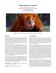
Figure 1: The searchlight problem consisting of a semiinfinite
planar homogeneous medium, a Fresnel boundary
and a focused pencil beam of light entering the media. The
pencil beam continues after the refraction as an exponentially
decaying linear source. The light is absorbed and scattered
and some of it exits the top boundary.
2.1. The BSSRDF and the Searchlight Problem
When rendering translucent materials, it is often convenient
to re-formulate this problem in analogy to the local surface
reflection integral. This results in an integral equation which
computes the outgoing radiance, L o, at position and direction
(⃗x o,⃗ω o) as a convolution of the incident illumination, L i , and
the BSSRDF, S, over all incident positions and directions
(⃗x i ,⃗ω i ):
∫ ∫
L o(⃗x o,⃗ω o)= S(⃗x i ,⃗ω i ;⃗x o,⃗ω o)L i (⃗x i ,⃗ω i )(⃗n ·⃗ω i ) d⃗ω i dA(⃗x i ). (2)
A
2π
The most general method to solve this integral is brute-force
Monte Carlo particle tracing. While this method is both general,
intuitive, and simple to implement, unfortunately it gives
noisy results and converges very slowly. Hence, researchers
in fields such as medical physics, astrophysics, and recently
computer graphics have developed alternative solution methods,
and usually only use brute-force Monte Carlo particle
tracing for validation.
For efficiency, S is often decomposed into reducedradiance,
single-scattering, and multi-scattering terms, S =
S (0) + S (1) + S d , so that each can be handled by specialized
algorithms. Most previous techniques in graphics have approximated
S (1) with the refractive single-scattering approximation
proposed by Jensen et al. [JMLH01] and we propose
an alternate diffuse single-scattering approximation [HCJ13].
Accurate brute-force simulation of the multi-scattering term
S d is as expensive as the general problem, so we rely on
simplifications to the multi-scattering problem based on approximate
solutions to the so-called “searchlight problem.”
The searchlight problem, illustrated in Figure 1, considers
a simplified setting where a focused pencil beam of unit
flux is orthogonally incident at the origin on a semi-infinite
planar homogeneous medium. Photons refract through a Fresnel
boundary and travel in the downward direction until
∞
they are scattered or absorbed by the medium. The unabsorbed/unscattered
photons form an exponentially decaying
linear source inside the medium. The scattered photons can
be scattered again and ultimately get absorbed or escape the
medium. The sum of all photons exiting the upper boundary
at each point⃗x forms a spatial diffuse reflectance profile R d (⃗x),
which is radially symmetric (1D) for normally-incident light,
R d (⃗x) = R d (‖⃗x‖). Even though the searchlight problem is simpler
than the fully general setting, exact solutions only exist
for special cases—we still rely on brute-force Monte Carlo
particle tracing for validation, just as for the general problem.
Most methods in graphics simplify S d as a product of a
typically 1D, diffuse reflectance profile R d and a directional,
energy-preserving Fresnel reshaping term [JMLH01, dI11]:
S d (⃗x i ,⃗ω i ;⃗x o,⃗ω o) = 1 π Ft(⃗x i,⃗ω i ,η)R d (⃗x o −⃗x i ) Ft(⃗xo,⃗ωo,η) , (3)
4C φ (1/η)
where the reflectance profile is now centered at the incident
light position, ⃗x i , and 4C φ is a constant needed for normalization.
To evaluate this expression efficiently, most methods
have relied on diffusion theory to obtain an analytic approximation
for R d .
3. Classical Diffusion Theory
3.1. The Classical Diffusion Equation
The classical diffusion approximation solves Equation (1) by
considering only a first-order spherical harmonic expansion
of the radiance:
L(⃗x,⃗ω) ≈ 1
4π φ(⃗x) + 3
4π ⃗ E(⃗x) ·⃗ω, (4)
where the fluence φ and vector flux ⃗E are the first two angular
moments of the radiance distribution:
∫
∫
φ(⃗x) = L(⃗x,⃗ω) d⃗ω, ⃗E(⃗x) = L(⃗x,⃗ω)⃗ω d⃗ω. (5)
4π
4π
If we further assume that the source function Q is isotropic,
the classical diffusion equation follows from this approximation:
−D∇ 2 φ(⃗x) + σ aφ(⃗x) = Q(⃗x), (6)
where D = 1/3σ t
′ is the diffusion coefficient and σ t ′ is the reduced
extinction coefficient obtained by applying similarity
theory with σ t ′ = (1 − g)σ s + σ a. In the case of a unit power
isotropic point source (a monopole) in an infinite homogeneous
medium, the solution to Equation (6) is the classical
diffusion Green’s function:
φ m (⃗x) = 1
4πD
e −σtrd(⃗x)
d(⃗x)
, (7)
where σ tr = √ σ a/D is the transport coefficient and d(⃗x) is the
distance from ⃗x to the point source. We use the superscript on
φ m to indicate fluence from a monopole.

R. Habel, P. Christensen & W. Jarosz / Classical and Improved Diffusion Theory for Subsurface Scattering
3.2. Obtaining the Diffusion Profile
The Source Function. To render subsurface scattering, a
suitable source function needs to be defined. In reality, each
ray of light incident on a smooth surface gives rise to a refracted
ray within the medium with exponentially decreasing
intensity. To avoid integrating from this extended beam
source, Farrell et al. [FPW92] proposed concentrating all the
light at the center of mass of the beam (a depth of one mean
free path (1/σ ′ t
) inside the medium), effectively replacing the
beam source with a single isotropic point source inside the
medium. This single-depth approximation was later adopted
by Jensen et al. [JMLH01].
Boundary Conditions. For semi-infinite configurations, the
boundary condition can be handled in an approximate fashion
with the “method of images” by placing a mirrored negative
source outside the medium for every positive source inside
the medium. The mirroring is performed above an extrapolated
boundary such that the fluence is zero at a distance
z b = 2AD above the surface. This offset takes into account
the index of refraction mismatch at the boundary through
the reflection parameter A. Jensen et al. [JMLH01] used
where η is the relative index of refraction
at the surface and C i is the i th angular moment of the Fresnel
function. Analytic solution to the angular moments are
defined by Aronson [Aro95]. Approximations to the angular
moments, including constant factors used in the calculations
(2 for C 1 (η) and 3 for C 2 (η)), are provided by d’Eon and
Irving [dI11]:
A(η) ≈ 1+2C 1(η)
1−2C 1 (η)
⎧
0.919317 − 3.4793η + 6.75335η 2
⎪⎨ −7.80989η 3 + 4.98554η 4 − 1.36881η 5 , η < 1
2C 1 (η)≈
(8)
−9.23372 + 22.2272η − 20.9292η 2
⎪⎩
+10.2291η 3 − 2.54396η 4 + 0.254913η 5 , η ≥ 1
⎧
0.828421 − 2.62051η + 3.36231η 2
−1.95284η 3 + 0.236494η 4 + 0.145787η 5 , η < 1
⎪⎨
3C 2 (η)≈
−1641.1 + 135.926η −3 − 656.175η −2 (9)
+1376.53η −1 + 1213.67η − 568.556η 2
⎪⎩
+164.798η 3 − 27.0181η 4 + 1.91826η 5 , η ≥ 1.
The Dipole. The single-depth approximation, together with
the method of images to satisfy the boundary conditions,
forms a dipole consisting of a positive and negative monopole
pair from Equation (7):
φ d (⃗x) = 1
4πD
(
e −σtrd(⃗x,⃗xr)
d(⃗x,⃗x r)
)
− e−σtrd(⃗x,⃗xv)
d(⃗x,⃗x v)
(10)
where d(⃗x a,⃗x b ) is the distance between two points, the real
source at ⃗x r is at a depth z r = 1/σ t
′ within the medium (regardless
of incident light direction), and the mirrored virtual
source at ⃗x v = (−⃗x r + 2z b ⃗n) is placed at a height z v = z r + 2z b
above the surface. We use the superscript on φ d to indicate
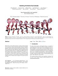
fluence due to a dipole. Figure 2 illustrates the resulting configuration.
d v
d r
Figure 2: The single-depth approximation replaces the extended
beam source with a single isotropic point source
(green) at a depth z r inside the medium. This source is mirrored
about an extrapolated boundary z b above the surface,
creating a negative point source (red) outside of the medium.
Diffuse Reflectance Profile. The equations so far have expressed
the fluence volumetrically within the medium. To
render surfaces, however, we wish to compute the light leaving
various points on the boundary.
To handle this, Jensen et al. [JMLH01] used Fick’s law
which states that (for isotropic sources) the vector flux is the
gradient of the fluence:
z r
∞
⃗E(⃗x) = −D⃗∇φ(⃗x). (11)
Since the radiant exitance on the boundary is the dot product
of the vector flux with the surface normal, we have † :
R d (⃗x) = ⃗E(⃗x) ·⃗n = −D(⃗∇ ·⃗n)φ(⃗x). (12)
Hence, to compute the diffusion profile R d (⃗x) due to a dipole,
we need to evaluate the directional derivative (⃗∇ ·⃗n) of the
fluence (10) in the direction of the normal. This gives us:
[
R d (⃗x)= α′ zr (1 + σ trd r)e −σtrdr
4π dr
3
z b
zv (1 + σtrdv)e−σtrdv
+
dv
3
]
, (13)
where we use the shorthand d r = d(⃗x,⃗x r) and d v = d(⃗x,⃗x v).
In classical diffusion theory, the diffuse reflectance profile
R d (⃗x) in Equation (12) depends only on the surface flux (the
gradient of the fluence along the surface normal) and not
the fluence φ(⃗x) itself due to Fick’s law. In more general
† Note that since the searchlight problem assumes incident light
of unit flux (power), the diffuse reflectance profile R d (⃗x) actually
expresses the radiant exitance [Wm −2 ] response normalized per unit
incident flux [W], resulting in units of [m −2 ] for R d (⃗x).

R. Habel, P. Christensen & W. Jarosz / Classical and Improved Diffusion Theory for Subsurface Scattering
terms, this applies Neumann boundary conditions where only
derivatives are specified. This can be formally expressed as:
R d (⃗x) = C φ φ(⃗x) +C ⃗ E (−D( ⃗∇ ·⃗n)φ(⃗x)). (14)
with factors C φ = 0 and C ⃗ E = 1 so only vector flux, and not
fluence, contributes to the diffuse reflectance. These relative
contributions change with other exitance calculations (other
boundary conditions) as we will discuss in the next section.
4. Improved Diffusion Theory
D’Eon and Irving [dI11] introduced a wealth of improvements
for diffusion theory from other fields such as medical
physics and astrophysics to computer graphics, including
a modified diffusion equation, a more accurate reflection
parameter A, and a more accurate exitance calculation. We
summarize these changes here, and in doing so we will introduce
new terms for the aforementioned expressions with a
subscript G.
4.1. Grosjean’s Diffusion Equation
Grosjean [Gro56, Gro58] proposed a different approximation
for the fluence due to an isotropic point source (monopole)
in an infinite medium,
φ m G (⃗x) = e−σ′ t d(⃗x)
4πd 2 (⃗x) + α′ e −σ tr,Gd(⃗x)
. (15)
4πD G d(⃗x)
This is the sum of the exact single scattering and approximate
multi scattering using Grosjean’s modified diffusion
coefficient
D G = 2σa + σ′ s
3σ ′2 t
= 1
3σ ′ t
+ σa
3σ t
′2
, (16)
and the transport coefficient is defined in the same way as in
classical diffusion σ tr,G = √ σ a/D G , but using this modified
diffusion coefficient D G .
The single-scattering term is not considered part of the
diffusion theory and is therefore handled separately. In contrast
to classical diffusion theory, this explicitly excludes
single scattering from the diffusion approximation. Single
scattering can be calculated exactly using Monte Carlo methods
[WZHB09, JC98, DJ07, JNSJ11], or it can be approximated
[JMLH01, HCJ13].
Grosjean’s approximation gives rise to a modified diffusion
equation:
−D G ∇ 2 φ(⃗x) + σ aφ(⃗x) = α ′ Q(⃗x). (17)
Compared to Equation (6), this diffusion equation multiplies
the source term by the reduced albedo α ′ . This multiplication
is a result of the exclusion of single scattering, which provides
more accurate solutions near the source and for low albedos.
The Green’s function of Equation (17) is the second term of
Equation (15) which likewise has an additional albedo term
compared to the classical diffusion Green’s function (7).
Boundary Conditions. To handle the surface boundary,
D’Eon and Irving still use the same boundary condition where
fluence is forced to zero at a distance z b = 2A G D G , but use
Grosjean’s D G (16) and an improved reflection parameter,
A G (η) ≈ 1+3C 2(η)
1−2C 1 (η) [PG95].
Improved Dipole. With these changes, the fluence due to
a dipole defined with the single-depth approximation and
method of images is [d’E12]:
(
)
φ d α′ e −σ tr,Gd(⃗x,⃗x r)
G (⃗x,⃗xr) = − e−σ tr,Gd(⃗x,⃗x v)
, (18)
4πD G d(⃗x,⃗x r) d(⃗x,⃗x v)
where, compared to Equation (10), the additional α ′ takes
the single-scattering separation into account. Please note that
we call this the “improved dipole” rather than the “better
dipole” [d’E12] for naming consistency.
Radiant Exitance. Instead of using Fick’s Law, which relies
solely on vector flux, d’Eon and Irving use a Robin boundary
condition introduced by Kienle and Patterson [Aro95, KP97]
which uses a linear combination of the fluence and its derivative,
the vector flux. The result is a more accurate radiant
exitance, defined as in Equation (14):
R d,G (⃗x) = C φ,G φ(⃗x) +C ⃗ E,G (−D( ⃗∇ ·⃗n)φ(⃗x)), (19)
but where C φ,G = 1 4 (1−2C 1(η)) and C ⃗ E,G = 1 2 (1−3C 2(η)). Evaluating
the fluence contribution together with the vector flux
gives us:
with ‡
R d,G (⃗x) = R φ d,G (⃗x) + R⃗ E
d,G (⃗x) (20)
(
)
R φ d,G (⃗x) = C α ′2 e −σ tr,Gd r
φ,G
− e−σ tr,Gd v
, and (21)
4πD G d r d v
[ ( )
R ⃗ E α ′2 zr 1 + σtr,G d r e −σ tr,G d r
d,G (⃗x) = C ⃗ E,G
4π
dr
3 + (22)
(z r + 2z b ) ( ) ]
1 + σ tr,G d v e −σ tr,G d v
dv
3 ,
again using the shorthand d r = d(⃗x,⃗x r) and analogously for d v,
and where z r = 1/σ ′ t
is the fixed depth of the real source.
The improved diffusion theory consistently delivers better
results than the classical theory and should therefore be preferred
for computer graphics purposes. Table 2 summarizes
and compares important quantities from both diffusion theories.
All other parameters such as the dipole depth z b or the
transport coefficient σ tr follow from these definitions.
4.2. Extended Source
Accounting for the entire beam of photons entering the
medium requires defining an extended source along the (re-
‡ Formulas corrected Sept. 2013

R. Habel, P. Christensen & W. Jarosz / Classical and Improved Diffusion Theory for Subsurface Scattering
Table 2: Comparison of classical and improved diffusion model
Term Classical Diffusion Improved Diffusion
Diffusion Equation −D∇ 2 φ(⃗x) + σ aφ(⃗x) = Q(⃗x) −D G ∇ 2 φ(⃗x) + σ aφ(⃗x) = α ′ Q(⃗x)
Green’s Function Isotropic Source φ m (⃗x) = 1 e −σtrd(⃗x)
φ 4πD d(⃗x) m α′ e
G (⃗x) = −σ tr,G d(⃗x)
4πD G d(⃗x)
Diffusion Coefficient D = 1
3σ ′ t
Reflection Parameter
A(η) = 1+2C 1(η)
1−2C 1 (η)
D G = 2σa+σ′ s
3σ ′2 t
= 1
3σ ′ t
A G (η) = 1+3C 2(η)
1−2C 1 (η)
+ σa
3σ ′2 t
Exitance Parameter Fluence C φ = 0 C φ,G = 1 4 (1 − 2C 1(η))
Exitance Parameter Flux C ⃗ E = 1 C ⃗E,G = 1 2 (1 − 3C 2(η))
fracted) beam, with an exponential falloff formed by all firstscatter
events inside the medium [FPW92]:
Q(t) = α ′ σ ′ t e−σ′ t t , (23)
where t is the distance along the source beam inside the
medium.
Radiant Exitance from Extended Source. Obtaining the
fluence due to the extended source in a semi-infinite medium
requires sweeping the Green’s function along the beam:
∫ ∞
φ b (⃗x,⃗ω) = φ d (⃗x,⃗x r(t))Q(t) dt, (24)
0
where φ d (⃗x r(t)) is the dipole Green’s function (18) with the
previously constant position of the real source ⃗x r now varying
along the beam ⃗x r(t) = t⃗ω. Note that this creates a positive
as well as a mirrored negative extended source due to the
method of images for handling the semi-infinite medium.
ω
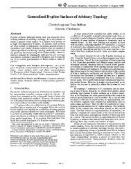
Figure 3: The extended source is created by sweeping the
dipole Green’s function along the beam direction ⃗ω. Due to
the method of images, a corresponding negative extended
source is created.
∞
z b
We use the superscript on φ b to denote fluence from a beam
source. The resulting configuration is depicted in Figure 3.
This step is independent of the underlying diffusion theory
and can be performed with any Green’s function and exitance
calculations, but due to its superiority, we only show the
derivation for the improved diffusion theory.
To obtain the diffuse reflectance profile on the surface we
need to instead integrate Equation (19) over the beam. This
results in the integral
∫ ∞
R d,G (⃗x,⃗ω) = r(⃗x,⃗x r(t))Q(t) dt, (25)
0
where r(⃗x,⃗x r(t)) = R φ d,G (⃗x,t) + R⃗ E
d,G (⃗x,t) with:
(
)
R φ d,G (⃗x,t) = C α ′ e −σ tr,Gd r(t)
φ,G
− e−σ tr,Gd v(t)
, and (26)
4πD G d r(t) d v(t)
[
R ⃗ E α ( ′ zr(t) 1 + σ tr,G d ) r(t) e −σ tr,Gd r(t)
d,G (⃗x,t) = C ⃗ E,G
4π
dr 3 + (27)
(t)
(z r(t) + 2z b ) ( 1 + σ tr,G d ) ]
v(t) e −σ tr,Gd v(t)
dv 3(t) ,
using the shorthand d r(t) = d(⃗x,⃗x r(t)) and analogously for d v,
and where z r(t) =⃗x r(t) ·⃗n is the depth of the real source. This
redefines R φ d,G (⃗x) and R⃗ E
d,G (⃗x) from the single-depth approximation
(21–22) to be dependent on the depth of a point t on
the extended source.
5. Solving the Extended Source
D’Eon and Irving [dI11] noted that Equation (25) has no
closed-form solution, and proposed to approximate it using a
sum of Gaussians:
R d (⃗x) ≈ α ′ k−1
∑ (w R (i)w i ) G 2D (v i ,x), (28)
i=0
where x = ‖⃗x‖, (w R (i)w i ) are the weights, and v i are the variances
of normalized 2D Gaussians G 2D . The equations necessary
to obtain the weights and variances of the Gaussians are

R. Habel, P. Christensen & W. Jarosz / Classical and Improved Diffusion Theory for Subsurface Scattering
themselves fairly complex summations of integrals depending
on further weights w φR (v,i),w ⃗ ER (v,i).
In our recent article [HCJ13], we showed that it is efficient
to numerically approximate Equation (25) using Monte Carlo
integration with exponential and equiangular importance sampling
[KF12, NNDJ12]. We further increased the accuracy of
the improved diffusion model using an empirical correction
factor.
6. Conclusion
This technical report has provided an overview of classical
and improved diffusion theory, independent of any solution
methods. So far, two solution methods have been used: quantized
diffusion [dI11] and Monte Carlo integration [HCJ13],
and it is our hope that this overview of diffusion theory might
inspire other solution methods in the future.
[KF12] KULLA C., FAJARDO M.: Importance sampling techniques
for path tracing in participating media. Computer Graphics
Forum (Proc. Eurographics Symposium on Rendering) 31, 4
(2012), 1519–1528. 6
[KP97] KIENLE A., PATTERSON M. S.: Improved solutions of
the steady-state and the time-resolved diffusion equations for
reflectance from a semi-infinite turbid medium. Journal of the
Optical Society of America A 14, 1 (1997), 246–254. 4
[NNDJ12] NOVÁK J., NOWROUZEZAHRAI D., DACHSBACHER
C., JAROSZ W.: Virtual ray lights for rendering scenes with
participating media. ACM Transactions on Graphics (Proc. SIG-
GRAPH) 31, 4 (2012), 60:1–60:11. 6
[PG95] POMRANING G. C., GANAPOL B. D.: Asymptotically
consistent reflection boundary conditions for diffusion theory.
Annals of Nuclear Energy 22, 12 (1995), 787–817. 4
[WZHB09] WALTER B., ZHAO S., HOLZSCHUCH N., BALA K.:
Single scattering in refractive media with triangle mesh boundaries.
ACM Transactions on Graphics (Proc. SIGGRAPH) 28, 3
(2009). 4
References
[Aro95] ARONSON R.: Boundary conditions for diffusion of light.
Journal of the Optical Society of America A 12, 11 (1995), 2532–
2539. 3, 4
[Cha60] CHANDRASEKAR S.: Radiative Transfer. Dover, 1960. 1
[d’E12] D’EON E.: A better dipole. Tech. rep., http://www.-
eugenedeon.com, 2012. 4
[dI11] D’EON E., IRVING G.: A quantized-diffusion model for
rendering translucent materials. ACM Transactions on Graphics
(Proc. SIGGRAPH) 30, 4 (2011), 56:1–56:14. 1, 2, 3, 4, 5, 6
[DJ07] DONNER C., JENSEN H. W.: Rendering translucent materials
using photon diffusion. Rendering Techniques (Proc. Eurographics
Symposium on Rendering) (2007), 243–252. 4
[FPW92] FARRELL T. J., PATTERSON M. S., WILSON B.: A
diffusion theory model of spatially resolved, steady-state diffuse
reflectance for the noninvasive determination of tissue optical
properties in vivo. Medical Physics 19, 4 (1992), 879–888. 3, 5
[Gro56] GROSJEAN C. C.: A high accuracy approximation for
solving multiple scattering problems in infinite homogeneous
media. Il Nuovo Cimento (1955-1965) 3 (1956), 1262–1275. 4
[Gro58] GROSJEAN C. C.: Multiple isotropic scattering in convex
homogeneous media bounded by vacuum. In Proc. Second
International Conference on the Peaceful Uses of Atomic Energy
(1958), vol. 413. 4
[HCJ13] HABEL R., CHRISTENSEN P. H., JAROSZ W.: Photon
beam diffusion: A hybrid Monte Carlo method for subsurface
scattering. Computer Graphics Forum (Proc. Eurographics Symposium
on Rendering) 32, 4 (June 2013). 1, 2, 4, 6
[JC98] JENSEN H. W., CHRISTENSEN P. H.: Efficient simulation
of light transport in scenes with participating media using photon
maps. Computer Graphics (Proc. SIGGRAPH) 32 (1998), 311–
320. 4
[JMLH01] JENSEN H. W., MARSCHNER S. R., LEVOY M., HAN-
RAHAN P.: A practical model for subsurface light transport. Computer
Graphics (Proc. SIGGRAPH) 35 (2001), 511–518. 2, 3,
4
[JNSJ11] JAROSZ W., NOWROUZEZAHRAI D., SADEGHI I.,
JENSEN H. W.: A comprehensive theory of volumetric radiance
estimation using photon points and beams. ACM Transactions on
Graphics 30, 1 (2011), 5:1–5:19. 4