Lectures on Elementary Probability

3.3. JOINT PROBABILITY MASS FUNCTIONS 19
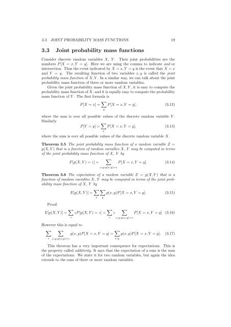
3.3 Joint probability mass functions
Consider discrete random variables X, Y . Their joint probabilities are the
numbers P [X = x, Y = y]. Here we are using the comma to indicate and or
intersection. Thus the event indicated by X = x, Y = y is the event that X = x
and Y = y. The resulting function of two variables x, y is called the joint
probability mass function of X, Y . In a similar way, we can talk about the joint
probability mass function of three or more random variables.
Given the joint probability mass function of X, Y , it is easy to compute the
probability mass function of X, and it is equally easy to compute the probability
mass function of Y . The first formula is
P [X = x] = ∑ y
P [X = x, Y = y], (3.12)
where the sum is over all possible values of the discrete random variable Y .
Similarly
P [Y = y] = ∑ P [X = x, Y = y], (3.13)
x
where the sum is over all possible values of the discrete random variable X.
Theorem 3.5 The joint probability mass function of a random variable Z =
g(X, Y ) that is a function of random variables X, Y may be computed in terms
of the joint probability mass function of X, Y by
∑
P [g(X, Y ) = z] = P [X = x, Y = y]. (3.14)
x,y:g(x,y)=z
Theorem 3.6 The expectation of a random variable Z = g(X, Y ) that is a
function of random variables X, Y may be computed in terms of the joint probability
mass function of X, Y by
E[g(X, Y )] = ∑ ∑
g(x, y)P [X = x, Y = y]. (3.15)
x y
Proof:
E[g(X, Y )] = ∑ z
zP [g(X, Y ) = z] = ∑ z
∑
z P [X = x, Y = y] (3.16)
x,y:g(x,y)=z
However this is equal to
∑ ∑
z
x,y:g(x,y)=z
g(x, y)P [X = x, Y = y] = ∑ x,y
g(x, y)P [X = x, Y = y]. (3.17)
This theorem has a very important consequence for expectations. This is
the property called additivity. It says that the expectation of a sum is the sum
of the expectations. We state it for two random variables, but again the idea
extends to the sum of three or more random variables.