Lectures on Elementary Probability

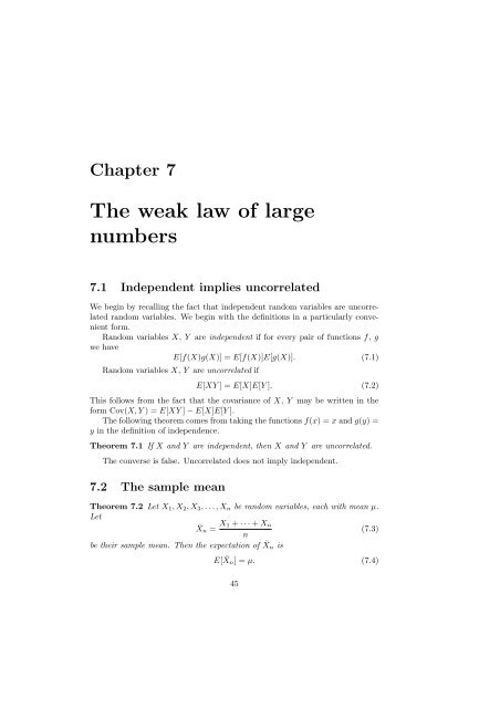
Chapter 7
The weak law of large
numbers
7.1 Independent implies uncorrelated
We begin by recalling the fact that independent random variables are uncorrelated
random variables. We begin with the definitions in a particularly convenient
form.
Random variables X, Y are independent if for every pair of functions f, g
we have
E[f(X)g(X)] = E[f(X)]E[g(X)]. (7.1)
Random variables X, Y are uncorrelated if
E[XY ] = E[X]E[Y ]. (7.2)
This follows from the fact that the covariance of X, Y may be written in the
form Cov(X, Y ) = E[XY ] − E[X]E[Y ].
The following theorem comes from taking the functions f(x) = x and g(y) =
y in the definition of independence.
Theorem 7.1 If X and Y are independent, then X and Y are uncorrelated.
The converse is false. Uncorrelated does not imply independent.
7.2 The sample mean
Theorem 7.2 Let X 1 , X 2 , X 3 , . . . , X n be random variables, each with mean µ.
Let
¯X n = X 1 + · · · + X n
(7.3)
n
be their sample mean. Then the expectation of ¯Xn is
E[ ¯X n ] = µ. (7.4)
45