Lectures on Elementary Probability

More documents

Recommendations

Info

$Math 520a - Midterm take home exam Do 5 out of the 6 problems ...$

$page 1 of 2 Math 410 Matrix Analysis Fall 2007 Final Exam Answers ...$

26 CHAPTER 4. THE BERNOULLI PROCESS Now take the limit as n → ∞ and p → 0 with λ = np fixed. The first factor does not depend on n. The second factor goes to one. The third factor has limit e −λ . The fourth factor goes to one. So the result is P [N = k] = λk k! e−λ . (4.15) This is the Poisson probability formula. Here is some more detail on the limits. The quotient (n) k divided by n k may be computed by dividing each of the k factors in (n) k by n. Then the limit of each of the resulting k factors is one. So the limit of the product is one. This is reasonable. The (n) k is the number of ordered samples without replacement of size k from a population of size n. The n k is the number of ordered samples with replacement of size k from a population of size n. It is reasonable that for a very large population the two methods of sampling give equivalent results. The limit of (1 − λ/n) n may be computed by using properties of logarithms. The Taylor series of 1/(1 − x) = 1 + x + x 2 + x 3 + · · ·, the geometric series. Therefore, by integrating, the Taylor series of the logarithm is − ln(1 − x) = x+x 2 /2+x 3 /3+x 4 /4+· · ·, the integral of the geometric series. The logarithm of (1 − λ/n) n is n ln(1 − λ/n). Expand the logarithm in a Taylor series. This gives −n[λ/n + (1/2)λ 2 /n 2 + · · ·]. Multiply out. This gives −[λ + (1/2)λ 2 /n + · · ·]. This shows that as n → ∞ the limit of the logarithm of (1 − λ/n) n is −λ. Since the exponential is the inverse function of the logarithm, the limit as n → ∞ of (1 − λ/n) n is e −λ . Note that in this chapter the parameter λ is dimensionless and has the interpretation of the mean of the Poisson probability. The variance is also λ. Therefore the standard deviation is √ λ. When λ is large, then the standard deviation is small relative relative to the mean. Thus for large λ the Poisson distribution is peaked around the mean, at least in a relative sense. 4.5 Geometric random variables Consider a Bernoulli process with parameter p > 0. Let W be the trial on which the first success occurs. Then the probability of the event that W = n is the probability of a pattern of n − 1 failures followed by a success. This kind of random variable is called geometric. This proves the following theorem. Theorem 4.4 For a geometric random variable W with parameter p the distribution is given for n = 1, 2, 3, . . . by P [W = n] = P [N n−1 = 0]P [X n = 1] = (1 − p) n−1 p. (4.16) Theorem 4.5 The expectation of the geometric random variable is E[W ] = 1 p . (4.17)
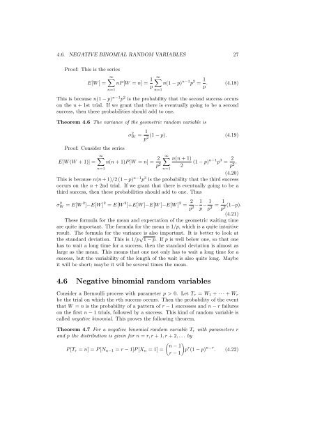
4.6. NEGATIVE BINOMIAL RANDOM VARIABLES 27 Proof: This is the series ∞∑ E[W ] = nP [W = n] = 1 ∞∑ n(1 − p) n−1 p 2 = 1 p p . (4.18) n=1 This is because n(1 − p) n−1 p 2 is the probability that the second success occurs on the n + 1st trial. If we grant that there is eventually going to be a second success, then these probabilities should add to one. n=1 Theorem 4.6 The variance of the geometric random variable is Proof: Consider the series ∞∑ E[W (W + 1)] = n(n + 1)P [W = n] = 2 p 2 n=1 σW 2 = 1 (1 − p). (4.19) p2 ∞ ∑ n=1 n(n + 1) 2 (1 − p) n−1 p 3 = 2 p 2 . (4.20) This is because n(n + 1)/2 (1 − p) n−1 p 3 is the probability that the third success occurs on the n + 2nd trial. If we grant that there is eventually going to be a third success, then these probabilities should add to one. Thus σ 2 W = E[W 2 ]−E[W ] 2 = E[W 2 ]+E[W ]−E[W ]−E[W ] 2 = 2 p 2 −1 p − 1 p 2 = 1 p 2 (1−p). (4.21) These formula for the mean and expectation of the geometric waiting time are quite important. The formula for the mean is 1/p, which is a quite intuitive result. The formula for the variance is also important. It is better to look at the standard deviation. This is 1/p √ 1 − p. If p is well below one, so that one has to wait a long time for a success, then the standard deviation is almost as large as the mean. This means that one not only has to wait a long time for a success, but the variability of the length of the wait is also quite long. Maybe it will be short; maybe it will be several times the mean. 4.6 Negative binomial random variables Consider a Bernoulli process with parameter p > 0. Let T r = W 1 + · · · + W r be the trial on which the rth success occurs. Then the probability of the event that W = n is the probability of a pattern of r − 1 successes and n − r failures on the first n − 1 trials, followed by a success. This kind of random variable is called negative binomial. This proves the following theorem. Theorem 4.7 For a negative binomial random variable T r with parameters r and p the distribution is given for n = r, r + 1, r + 2, . . . by ( ) n − 1 P [T r = n] = P [N n−1 = r − 1]P [X n = 1] = p r (1 − p) n−r . (4.22) r − 1
Page 1: Lectures on Elemen
Page 4 and 5: 4 CONTENTS 5.4 Uncorrelated random
Page 6 and 7: 6 CHAPTER 1. COMBINATORICS of trial
Page 8 and 9: 8 CHAPTER 1. COMBINATORICS injectiv
Page 10 and 11: 10 CHAPTER 2. PROBABILITY AXIOMS Th
Page 12 and 13: 12 CHAPTER 2. PROBABILITY AXIOMS ti
Page 14 and 15: 14 CHAPTER 2. PROBABILITY AXIOMS M
Page 16 and 17: 16 CHAPTER 2. PROBABILITY AXIOMS di
Page 18 and 19: 18 CHAPTER 3. DISCRETE RANDOM VARIA
Page 24 and 25: 24 CHAPTER 4. THE BERNOULLI PROCESS
Page 32 and 33: 32 CHAPTER 5. CONTINUOUS RANDOM VAR
Page 38 and 39: 38 CHAPTER 6. THE POISSON PROCESS T
Page 40 and 41: 40 CHAPTER 6. THE POISSON PROCESS P
Page 42 and 43: 42 CHAPTER 6. THE POISSON PROCESS P
Page 44 and 45: 44 CHAPTER 6. THE POISSON PROCESS r
Page 46 and 47: 46 CHAPTER 7. THE WEAK LAW OF LARGE
Page 52 and 53: 52 CHAPTER 8. THE CENTRAL LIMIT THE
Page 58 and 59: 58 CHAPTER 9. ESTIMATION estimate t
Page 60 and 61: 60 CHAPTER 9. ESTIMATION let F (t
Page 62: 62 CHAPTER 9. ESTIMATION 9.4 The Ko

Lectures on Elementary Probability

You also want an ePaper? Increase the reach of your titles

Delete template?

Save as template?