University of Groningen Groningen Growth and Development Centre ...

University of Groningen
Groningen Growth and
Development Centre
Brazil and Mexico’s Manufacturing Performance in
International Perspective, 1970-98
Research Memorandum GD-52
Nanno Mulder, Sylvie Montout and Luis Peres Lopes
RESEARCH
MEMORANDUM

Brazil and Mexico’s Manufacturing
Performance in International Perspective,
1970-1998
Research Memorandum GD-52
Nanno Mulder, Sylvie Montout and
Luis Peres Lopes
Groningen Growth and Development Centre
January 2002

Brazil and Mexico's Manufacturing Performance
in International Perspective, 1970-98
Nanno Mulder*, Sylvie Montout, and Luis Peres Lopes1
CEPII, University of Paris I, and University of Coimbra
Abstract
This paper studies the labour productivity performances of Brazil and Mexico in international
perspective by comparing them with the United States, one of the international productivity leaders,
during the period 1970-99. Brazil and Mexico are compared separately with the USA, in 1985 and
1988 respectively using the International Comparisons of Output and Productivity (ICOP) method.
With ICOP, detailed sectoral-specific conversion factors (unit value ratios, UVRs) are estimated to
express value added per person engaged in a common currency. Brazilian productivity was 43 per
cent of the US level in 1985 and that of Mexico 27 per cent of the US in 1988. The extrapolation to
the 1970-99 period shows that the productivity gaps of the Latin countries with the USA widened, in
particular in the 1980s. In the 1990s, Brazil managed to stabilise the productivity differential, whereas
Mexico continued to loose ground relative to the USA. The paper also checks the validity of the
benchmark results by confronting them with the national accounts. Moreover, the quality of the
extrapolations is assessed by comparing them with benchmark comparisons for 1975.
JEL codes: L6, O4
*
Corresponding author. Contact address:
CEPII
9, rue Georges Pitard
74740 Paris Cedex 15
Tel. (33) 1 53 68 55 38
Fax (33) 1 53 63 55 04
E-mail: Mulder@cepii.fr
1 Sylvie Montout is also affiliated to TEAM-CNRS of the University of Paris I, and Luis Peres is researcher at
the Economics Faculty, University de Coimbra (Portugal). The authors are grateful to Eduardo Pereira Nunes of
the IBGE for providing detailed production statistics of the Censo industrial – 1985, INEGI for similar data from
the XIII Censo industrial, Marcio Lopes for an update of the 1975 bilateral product matches, and Bart van Ark
and Angus Maddison for providing access to their worksheets of the 1975 Brazil/USA and Mexico/USA
comparisons and advice.

1. Introduction
The manufacturing sectors in Brazil and Mexico underwent large changes in the past two decades.
Until the mid-1980s, they were still highly protected against foreign competition, received large
subsidies and part of manufacturing was state-owned. The debt-crisis of the 1980s meant the
bankruptcy of these import substitution policies and marked the beginning of more outward-oriented
policies. In the late 1980s and 1990s, these policie s completely changed the institutional environment,
led to the privatisation of state enterprises, and reinforced competition. Moreover, foreign trade was
liberalised by reducing tariffs and eliminating quotas and licences. Both countries reinforc ed the ir
multilateral and in particular regional trade relations through free trade agreements. The increased
exposure to foreign competition on the home market and abroad provided an important stimulus for
firms to improve their productivity and cost performances. This process was reinforced by a large
influx of foreign direct investment.
This paper assesses whether the changed environment in these two countries in the past
decades has led to an improvement of their manufacturing performances in international perspective.
It complements other studies which only assessed performance over time. Although these latter studies
indicate changes in productivity, they fail to indicate how far each branch and industry in Brazil and
Mexico is from the "best practice" world-wide and how this productivity gap changed over time. We
present two level comparisons, comparing Brazil and Mexico separately with the USA – the
international technology leader -, for 1985 and 1988. The level comparisons are combined with time
series to assess changes in the productivity gaps between Brazil and Mexico on the one hand and the
United States on the other during the period 1970-99. In this paper we focus on labour productivity
due to the absence of reliable estimates for capital stocks in Brazil and Mexico.
First major trends are presented in employment, value added and labour productivity growth
the three countries in each of the three countries. Subsequently we present the methodology used to
compare output and productivity across countries. Section 4 presents the results of the comparisons
for our benchmark years 1985 and 1988 in terms of the product matches and their results. The
representativeness of the comparisons is assessed by confronting census estimates of value added and
employment with those of the national accounts (section 5). The labour productivity results are
presented for the benchmark years in section 6 and for the 1970-99 period in section 7. The
competitiveness of Brazil and Mexican manufacturing is assessed by combining productivity estimates
with labour compensation data in section 8 and section 9 concludes.
2. Manufacturing in Brazil, Mexico and the United States
Brazil, Mexico and the United States represent the largest economies of the Americas. Brazil and
Mexico are middle-income countries with manufacturing sectors that are still developing, whereas the
USA is a high-income country with a highly matured manufacturing sector. Brazil and Mexico are in
many ways comparable, not only in terms of size but also in terms of the industrial and macroeconomic
policies followed in the past decades. Both countries tried for a long time to develop their
industries by protecting them from foreign (and domestic) competition and the provision of massive
subsidies. The debt crisis in the 1980s marked the bankruptcy of these policies. Since the late 1980s
1

and in particular in the 1990s, both countries completely changed their policies: they privatised most
state enterprises, eliminated subsidies, and opened their borders for foreign products. Important acts
in terms of regional integration are the memberships of Mexico to NAFTA and Brazil to Mercosur.
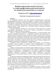
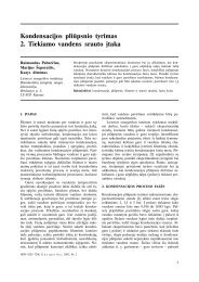
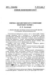
Figures 1 and 2 show some key characteristics of manufacturing in each country. Figure 1 shows the
composition of manufacturing value added by industry in Brazil, Mexico and United States from
1970-99. The composition of value added is relatively stable in the USA. In contrast, in Brazil and
Mexico important changes took place: the share of transport equipment increased mostly at the
expense of the shares of textiles and chemicals. Throughout the period the USA had smaller shares of
food products and textiles, and a larger share of machinery relative to Brazil and the USA.
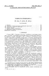
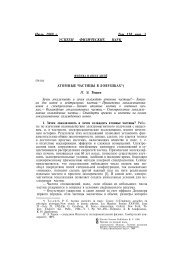
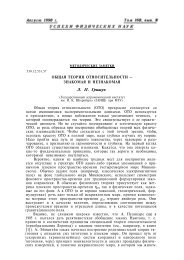
The main trends in output, employment and productivity growth in manufacturing in the 1970s
to 1990s are shown in Figure 2. Brazil and Mexico show very different trends compared to the USA,
in particular in terms of employment growth. During the entire 1970-99 period, the US experienced
positive output and labour productivity growth, even though these rates were relatively low in the
1970s. Productivity growth accelerated in the second half of the 1990s, in particular in machinery. 2
In contrast, Brazil and Mexico lived periods of up and downturns in employment and output growth.
Value added grew at relatively high rates in the 1970s and the 1990s. In the second half of the 1990s,
Mexico benefited from a increased demand from the USA which boosted its output growth. The most
important downturns in output growth were during the debt-crisis of the 1980s, in particular in Brazil.
Both countries show very different trends in employment growth. In Brazil, employment grew in the
1970s and between 1983 and 1989 and fell around 1980 and in the 1990s. In Mexic o, employment
growth was relatively constant over time, with a deceleration in the first half of the 1980s and
acceleration in the second half of the 1990s.
As Figure 2 illustrates, labour productivity growth was slightly higher in Mexican compared to
Brazilian manufacturing, except for food and transport equipment in which Brazil outperformed
Mexico. Both Latin countries showed significantly lower productivity growth than the USA. In
addition to growth rates, we should also take into account productivity levels. Some countries may
register high growth rates because they have low levels of productivity which allows them to benefit
from the large catch-up potential or productivity gap. This paper aims to check whether a link exists
between the growth rates and levels of productivity.
2 The spectacular productivity growth of this branch originates almost exclusively from the computer hardware
branch, which volume of production exploded due to rapid price declines. Employment remained almost
constant throughout the period, except for textiles and clothing which experienced a substantial decline.
2

Figure 1
Composition of Manufacturing Value Added by Industry at Current Prices
1970
100%
80%
60%
40%
20%
0%
Brazil Mexico USA
1985
100%
80%
60%
40%
20%
0%
Brazil Mexico USA
1998
100%
80%
60%
40%
20%
0%
Brazil Mexico USA
Food Textiles USA Wood, Paper
100% 0%
Chemicals Metals Machinery
Brazil Mexico USA
Transport Other
Sources: Brazil: Composition of Value Added by measure industry for 1970 and 85 from IBGE, Estatísticas
históricas do Brasil; 1998 from IBGE, Contas nacionais, 2001. Mexico for 1970, 1988 and 1999 from INEGI,
Sistema de cuentas nacionales, various editions. USA: BEA, National Income and Product Accounts, various
editions.
3

600
Figure 2
Indices of Value Added, Employment and Labour Productivity (1970=100)
Value Added Employment Labour Productivity
Brazil
600
600
500
500
500
400
400
400
Transport
300
Machinery
Food
Chemicals
Metals
Total
Other
300
Machinery
Textiles
300
Transport
200
200
Other
Total
Chemicals
Metals
Food
Transport
200
Wood, Paper
Food
Chemicals
Total
Metals
100
Textiles
100
100
Wood, Paper
Wood, Paper
Other
Machinery
Textiles
0
70 75 80 85 90 95
-
70 75 80 85 90 95
Mexico
-
70 75 80 85 90 95
600
Machinery
600
600
500
500
500
400
Transport
Chemicals
400
Transport
400
300
Total
Food
300
Machinery
300
200
100
Other
Metals
Textiles
Wood, Paper
200
100
Other
Total
Chemicals
Food
Textiles
Wood, Paper
Metals
200
100
Chemicals
Wood, Paper
Machinery
Metals
Total
Food
Transport
Textiles
Other
-
70 75 80 85 90 95
0
70 75 80 85 90 95
United States
-
70 75 80 85 90 95
600
Machinery
600
600
Machinery
500
500
500
400
400
400
300
200
100
Other
Transport
Metals
Chemicals
Total
Wood, Paper
Food
Textiles
300
200
100
Other
Total
Machinery
Wood, Paper
Food
Chemicals
Transport
Metals
300
200
100
Textiles
Total
Chemicals
Other
Metals
Food
Transport
Wood, Paper
-
70 75 80 85 90 95
-
70 75 80 85 90 95
Textiles
-
70 75 80 85 90 95
Sources: Brazil: 1970-85 from IBGE, Estatísticas históricas do Brasil; 1985-99 from IBGE, Contas nacionais,
various editions. Mexico: INEGI, Sistema de cuentas nacionales, various editions. USA: BEA, National Income
and Product Accounts. Value added for 1947-1987 is at fixed 1982 prices but is reweighted at current dollar
GPO every five years (1947, 1952, 1957, etc.). The series from 1987-1999 are chain weighted-series at 1992
dollars obtained from BEA (http://www.bea.doc.gov/bea/dn2.htm). Employment is full-time and part-time
employees plus self-employed
4

3. The ICOP Methodology
International comparisons of productivity levels is more complicated than intertemporal comparisons
of growth rates. Appropriate converters are required to express values of two or more countries in a
common currency. Exchange rates are unsuitable for this purpose, as they represent at best the relative
price of tradables, and not that of non-tradable sectors. Moreover, often they are not even
representative for relative prices of tradables, as the exchange rates tend to be affected by capital
movements, monetary policy and speculation.
Purchasing power parity (PPP) is an alternative conversion factor. There are two approaches to
estimate PPPs: (a) use of prices by category of final expenditure, and (b) comparison of producer
prices by sector of the economy. The former approach was followed in the International Comparisons
Project (ICP) (Kravis, Heston and Summers, 1982), and was also adopted by EUROSTAT and the
OECD. Benchmark expenditure PPPs are available for 1970, 1975, 1980, 1985, 1990 and 1993 and
1996.
Expenditure PPPs have been used as a proxy for producer prices in international productivity
comparisons by various authors. However, there are major objections to this approach. Firstly, ICP
PPPs are based on consumption prices of domestically produced goods AND imports, and exclude
goods produced for export. Secondly, ICP excludes price ratios of intermediate sectors which form a
substantial part of manufacturing output. Thirdly, expenditure PPPs are based on retail prices
including trade and transport margins. While these margins can be “peeled off” in theory, this
procedure poses many problems in practice. Fourthly, ICP PPPs are based on market prices. For the
comparison of production values, relative prices at factor costs are more relevant.
Another method to estimate PPPs is the so called international comparisons of output and productivity
(ICOP) approach. The origins of the production approach to international comparison stem from the
work of Rostas (1948) and Paige and Bombach (1959). It was further developed by the ICOP team at
the University of Groningen under the leadership of Angus Maddison. The first bilateral comparisons
for manufacturing were for Brazil/USA and Mexico/USA for 1975 and first published in 1988.
ICOP derives purchasing power parities from values of output and quantities produced by sector of the
economy. In combination with data on labour and capital, measures of labour, capital and total factor
productivity are compiled. Most ICOP comparisons have been bilateral, with the United States and
Germany as the numéraire countries, though multilateral techniques have also been applied to
manufacturing and agriculture comparisons. ICOP has focused mainly on agriculture and
manufacturing, although recently extensive work has also been done on services (see van Ark and
Timmer, 2001, for an overview of the ICOP work).
ICOP aims to develop industry-specific conversion factors using producer output data instead
of final expenditure information. This method is fundamentally different from the pricing technique in
the ICP expenditure approach. Ideally, one would like to use specific producer prices to develop
“industry PPPs”. However, no international comparable producer prices for specified products are
available. Instead ICOP uses product unit values which are derived from value and quantity
information for product groups. Hence each unit value has a quantity counterpart, as quantities times
"unit prices" equal the value equivalent. By matching as many products as possible, unit value ratios
5

are derived which can be weighted up to industry, branch and total manufacturing levels. These can
then be used to express output of different countries in a common currency.
One major advantage of the ICOP approach is that in general all necessary information can be
derived from a single primary source, which for manufacturing is the census of production or
industrial survey. This source contains great detail on the output and input structure by industry and
information on the sales values and quantities of most products. For Brazil, the data are derived from
the latest census of production for 1985 (Censos econômicos de 1985 – Censo industrial). We also
used production censuses for Mexico for 1988 (XIII Censo industrial - Censos económicos 1989) and
the United States for 1987 (1987 Census of Manufactures). The benchmark years were not only
chosen in relation to the latest production census in Brazil, but also because they are in the middle of
the period considered in this paper, i.e. 1970-99.
As the production censuses are not well harmonised across countries, the comparisons are
done on a two-country basis Brazil/USA and Mexico/USA. An advantage of comparing Brazil and
Mexico VIA the USA is that a comparison with the USA provides an indication of the productivity gap
between the countries and as such the potential of catch-up.
In the ICOP approach 3 , relative prices are referred to as unit value ratios (UVRs) instead of
PPPs as they are based on ratios of unit values (UVs) of products. These unit values are derived by
dividing ex-factory output values (o) by produced quantities (q) for each product i in each country:
o
i
UV
i
= (1)
qi
The unit value is a kind of average price at which a similar group of products was sold by all
manufacturers in a given year. In each bilateral comparison, products are matched according to more
or less detailed product descriptions, e.g. frozen fruits, infants' underwear, aluminium window frames,
and car tyres. For each matched product, the ratio of the unit values of both is calculated:
XU UV
UVR
i
= (2)
UV
X
i
U
i
with x being Brazil or Mexico and u the base country, the United States. The UVR indicates the
relative producer price of the matched product in both countries. Product UVRs are used to estimate
UVRs at more aggregate levels: industries, branches and total manufacturing. These levels correspond
to those distinguished in the 1987 US Standard Industrial Classification (SIC). Manufacturing output
is the sum of output of branches, which in turn is the sum of the industries’ output value. The value of
an industry's output equals the sum of the values of the produced products. Within the comparison of
each industry between two countries, only part of products can be matched as quantity information
often lacks, it may be difficult to find comparable products, or countries produce unique products.
The matched products can be considered as a sampled subset of products within an industry which
relative price, under certain conditions, may be considered representative for the non-matched part.
3 The description of the ICOP methodology is based on Timmer et al. (2001).
6

Aggregation Step One: from Product to Industry Level UVRs
The UVR for an industry is the weighted mean of the product UVRs, using output values of base
country (USA) or the other country (Brazil or Mexico) as weights. The UVR for an industry using US
weights is estimated as follows:
UVR
xu(
u)
j
I
= J
∑
i=
1
⎛UV
⎜
⎝UV
x(
x)
i
u(
u)
i
× w
with i=1,.,I J the matched products in industry j, w ij the output share of the ith commodity in industry j.
xu(u)
UVR
j
indicates the unit value ratio between country x and the base country (USA) weighted at
base country quantities indicated by the u in brackets. This equation can be rewritten to show that the
use of base country value weights leads to the Laspeyres index:
u(
u)
ij
⎞
⎟
⎠
with
w
u(
u)
ij
=
I
J
o
∑
i=
1
u(
u)
ij
o
u(
u)
ij
(3)
UVR
xu(
u)
j
=
I
J
∑
i=
1
I
J
∑
i=
1
q
q
u
ij
u
ij
* UV
* UV
x(
x)
ij
u(
u)
ij
(4)
Instead of US weights, one can also weight the product UVRs by the quantities of the "other" country
(Brazil or Mexico):
UVR
xu( x)
1
j
=
I x(
x)
J
∑
i=
1
⎛UVi
⎜
⎝UVi
u(
u)
× w
u(
x)
ij
⎞
⎟
⎠
with
w
u(
x)
ij
=
I
J
o
∑
i=
1
u(
x)
ij
o
u(
x)
ij
(5)
Again this index can be easily rewritten to show that it is a Paasche index:
UVR
xu(
x)
j
=
I
J
∑
i=
1
I
J
∑
i=
1
q
q
x
ij
x
ij
* UV
* UV
x(
x)
ij
u(
u)
ij
(6)
Aggregation Step Two: from Industry to Branch Level UVRs
The aggregation to branch UVRs is done by weighting the industry UVRs, by either US quantities:
UVR
xu(
u)
k
J
= k
x(
x)
⎛UV
⎟ ⎞
j
⎜
u(
u)
× w
jk
u(
u)
= 1⎝UVj
⎠
∑
j
(7)
with j=1,., J k the number of industries in branch k for which a UVR has been calculated (the
sample industries); w jk the output share of the j th industry in branch k. The weight of
industries depends not only on the size of their output but also on the reliability of the
industry UVR, being lower the lower the reliability, as unreliable UVRs should have a limited
influence on the branch UVR. Therefore the set of industries J k is split into two, J k (a) and
J k (b) depending on their reliability. UVRs of industries belonging to the first set (J k (a)) are
7

T u(u)
weighted with the total industry output at own prices: o
jk
. The UVRs from the other
industries (belonging to J k (b)) are weighted only by the output value of the matched products
in the industry:
o
M u(u)
jk
I j
∑
u u
= uv q . Hence the weights are given by
i=1
ij
ij
w
w
u(u)
jk
u(u)
jk
= o
= o
T u(u)
jk
M u(u)
jk
/ o
/ o
M u(u)
k
M u(u)
k
=
∀j∈
J
I j
∑
i=1
uv
u
ij
k
u
ij
(a)
q / o
M u(u)
k
∀j∈
J
k
(b)
(8)
with
o
M u(u)
k
=
T u(u)
∑ o
jk
+
J k (a)
∑
Jk
(b)
o
M u(u)
jk
To arrive at the Paasche index, the US weights are replaced by the Brazilian or Mexican output valued
at US prices:
UVR
xu( x)
1
k
=
J k
x(
x)
⎛UV
⎟ ⎟ ⎞
j
⎜
u(
x)
× w
jk
⎜ u(
u)
= 1⎝UVj
⎠
∑
j
(9)
with
w
w
u(x)
jk
u(x)
jk
= o
= o
T u(x)
jk
M u(x)
jk
/ o
/ o
M u(x)
k
M u(x)
k
I j
∑
i=1
∀j∈
J
uv
u
ij
x
ij
k
q / o
(a)
M u(x)
k
∀j∈
J
k
(b)
(10)
with
o
M u(x)
k
=
T u(x)
∑ o
jk
+
J k (a)
∑
Jk
(a )
o
M u(x)
jk
The split in the industry set is based on an assessment of the reliability of the industry UVRs.
Given the homogeneous character of the products belonging to an industry, it is expected that
product UVRs in an industry do not differ much. Hence, if the variation of the product UVRs
is high, this is an indication of unreliability. Also, reliability increases the higher the
percentage of industry output covered by matched products. Therefore the coverage ratio is
also taken into account when assessing the industry UVR reliability. The following decision
rule is used: when the coefficient of variation is less than 0.1, the industry is assigned to J k (a),
other wise to J k (b):
if
otherwise
[ ]
cv UVR
j
< 0.1
then
j∈
J
j∈
J
The coefficient of variation of industry j (cv j ) is measured as follows:
[ UVR ]
j
k
k
(a)
(b)
(11)
var
j
cv [ UVR ]
j
= (12)
UVR
The variance of the industry UVRs is given by the mean of the weighted deviations of the product
UVRs around the industry UVR (see Selvanathan, 1991):
8

I
1
= ∑
j
[ ] 1 − f ) w ( UVR −UVR
) 2
Var UVR
J
(
j)
ij ij
j
I
j
−1
i=
1
with Ij the number of products matched in industry i and f j the share of industry output which is
covered by the matched products within an industry. (1- f j ) is also referred to as the "finite population
correction", and ensures that an increase in the coverage of the sample reduces its variance. This
formula can be applied to either the Laspeyres or Paasche UVR using output value weights of the base
country for the variance of the Laspeyres, and quantity weights of the other country valued at US
prices for the variance of the Paasche. To allocate an industry to one of the two sets, a decision is
made on the basis of the (geometric) average variance for the Paasche and Laspeyres.
Aggregation Step Three: From Branch to Total Manufacturing UVRs
The aggregation of branch to total manufacturing UVRs is done in the same way as that from the
industry to the branch UVRs. US country output weights are used to arrive at the Laspeyres index,
and the Brazilian or Mexican quantities valued at US prices are used to arrive at the Paasche index.
The Laspeyres and Paasche indices are combined into a Fisher index when a single currency
conversion factor is required. It is defined as the geometric average of the Laspeyres and the Paasche.
There is one important difference between aggregation steps two and three, i.e. the output weights of
the branch do not depend on the reliability of their UVRs. Branches always enter the weighting
system with their total production. This is because the estimated UVRs are the most "characteristic"
for the branch even when their variance is high or their representativeness low. Nevertheless, it should
be stressed that the UVRs for this branch have to be interpreted with caution.
At the branch level, we can also estimate the reliability of the UVRs. As indicated by the stratified
sampling theory, branch variance is calculated by the quadratic output weighted average of the
corresponding industry UVRs:
(13)
J j
[
k
] = ( − f
k
) ∑ w
2 jk
var[ UVRjk
]
Var UVR
1 (14)
with f k the share of branch output covered by the matched products within a branch. Two variances are
estimated: one using US and one using "other" country weights, of which a geometric average is
taken.
Finally, the sample variance of the UVR for total manufacturing given by the quadratic output
weighted average of the corresponding branch UVR variances:
K
[ ] = ∑ w k
[ UVR k
]
Var UVR
k=
1
j=
1
2
var (15)
4. The Output and Productivity Comparisons: Matchings and UVRs
The first step in our two bilateral comparisons is the reconciliation of the industry nomenclatures of
Brazil and the USA on the one hand and Mexico and the USA on the other. This is done at the most
detailed industry level. As each country had its own industry classification in the 1980s which did not
correspond to an international classification, this was a difficult task. The most detailed breakdowns
of the Brazilian, Mexican and US censuses are in 530, 300, and 460 industries respectively. In the
Brazil/USA comparison, 229 common industries could be defined, and in the Mexico/USA
9

comparison 223 common industries. 4 These industries were regrouped into 19 different branches
according to the US Standard Industrial Classification 1987. We excluded branch 29 "Petroleum
refining and related industries", as it is strongly linked to the natural resource endowments of the
countries.
The second step consisted of matching products within each of the common industries in the
bilateral comparisons. An example is provided in Table 1 for branch 27 "Printing and Publishing" in
the Mexico/USA comparison. Within this branch, 4 common industries are defined. Within two
groups of industries (US 1987 SIC codes 27.41/51/52/53/54/59/61/71/82/89 and 27.91/93/95/96), it
was impossible to match any items. In industry group 2711/21, we were able to match one product,
and in industry 2731/32, six products were matched.
The UVRs of the product matches were aggregated in three steps, of which the first two are
illustrated in Tables 1 and 2 respectively. From the product to the industry level, the product UVRs
were weighted by either the US or the Mexican quantities. The second aggregation step from the
industry to the branch level is shown in Table 2, which recapitulates the UVRs of the industries of
Table 1. As in the industry groups 27.41/51/52/53/54/59/61/71/82/89 and 27.91/93/95/96 no
matchings could be made, their weight equals zero. For the common industry 27.11/21 with only one
match, no coefficient of variation could be derived. The weight of this industry equals the value of the
one matched product. In common industry 2731/32, several product were matched. As the coefficient
of variation of the UVRs is below 0.1, they are considered representative for the total industry.
Therefore the weight of this industry equals total output instead of the value of matched products (in
grey). If the coefficient would have been above 0.1, then only its matched output would have been
included in the weighting scheme. The "final" weights are converted to a common currency using the
industry UVRs of Table 1. Finally, the branch UVRs are obtained as shown in columns (11) to (13).
4 The correspondances of the industry nomenclatures are available upon request from the authors.
10

Table 1
Example of Aggregation Step 1: Printing and Publishing, Mexico/USA, 1987/88
US Product USA Mexico UVR of product matches
SIC matches Value Quantity Unit Value Quantity Unit At US At Fisher
(million (million) Value (million (million) Value weights Mexican
US$) pesos) weights
27 Printing, Publishing 7 8 670 476 000
27.11/21 Newspapers & periodicals 1 5 248 153 797 1 631 1 631 1 631
Newspapers 1 5 248 104 965 0,05 153 797 1 886 82 1 631 1 631 1 631
27.31/32 Books and book printing 6 3 422 322 203 1 315 1 252 1 283
Paperbound elementary school textbooks 511 116 4 21 400 4 4 933 1 114 1 114 1 114
Technical and bussiness books 1 272 105 12 85 727 5 17 580 1 450 1 450 1 450
Paperbound law books 149 6 27 53 750 2 28 342 1 045 1 045 1 045
Hardbound bibles 62 8 8 59 342 6 9 333 1 211 1 211 1 211
Other paperbound books 1 292 518 2 92 029 28 3 246 1 302 1 302 1 302
Pamphlets 135 115 1 9 955 7 1 487 1 271 1 271 1 271
27.41/51/52/53/54/59/61/71/82/89 0
27.91/93/95/96 0
Table 2
Example of Aggregation Step 2: Printing and Publishing, Mexico/USA, 1987/88
SIC Product Coefficient Matched Output Industry Output Final Weights Final UVRs
matches variation USA Mexico USA Mexico USA Mexico USA Mexico At US At Geo-
(geometric (million (million (mio. US$) (mio. pesos) (million (million (million (million weights Mexican metric
average) US$) pesos) US$) pesos) pesos) US$ ) weights average
(1) (2) (3) (4) (5) (6) (7) (8) (9) (10) (11) (12) (13)
(3) or = (4) or = (7) * = (8) / = =
(5)) (6)) US weights Mex. weights ((9)/(7)) ((8)/(10))
UVR) UVR)
27 7 0.001 8 670 476 000 65 055 617 837 21 124 617 837 29 432 162 465 1 393 1 329 1 361
27.11/21 1 5 248 153 797 49 179 1 225 601 5 248 153 797 8 560 729 94 1 631 1 631 1 631
27.31/32 6 0.047 3 422 322 203 15 876 464 040 15 876 464 040 20 871 433 371 1 315 1 252 1 283
27.41/51/52/53/54/59/61/71/82/89 66 984 1 408 829
27.91/93/95/96 4 157 475 990
11

The main results for the product matches, UVRs and reliability indicators are shown in Tables
3 and 4. Overall it was possible to match more than twice as many products between Mexico and the
USA than between Brazil and the USA, i.e. 435 instead of 209. In the Brazil/USA comparison, for
122 common industries it was impossible to match any products, in 56 industries it was possible to
match one product, in 27 industries two products, in 10 industries three products, in 10 industries four
products and in 4 industries five or more products. In the Mexico/USA comparison, in 61 common
industries it was impossible to match any products, in 40 industries it was possible to match one
product, in 42 industries two products, in 41 industries three products, in 19 industries four products
and in 20 industries five or more products. In both bilateral comparisons, most matches were made in
food products and machinery and computers. Other branches with many matchings in the Brazil/USA
comparison are furniture and fixtures and primary metals and metal products, and in the Mexico/USA
comparison electronic and electrical equipment, and textiles and wearing apparel.
The 1987 US census volumes and unit values were adjusted to make them comparable with
those for Brazil (1985) and Mexico (1988). From various issues of the US Industrial Outlook , it was
possible to derive producer price indices of the gross value of output at the most detailed (4-digit)
industry level for 1985 to 1988. From the Annual Survey of Manufactures, we obtained the gross
value of output and employment at the industry level for 1985 and 1988. With these data, the unit
value (p) and volume adjustment (q) factors were estimated. Subsequently, they are applied to the
Laspeyres index (see formulae (4)):
I
J
∑
i=
1
I
u,1975
x(
x)
qij
* q*
UVij
i= 1
(16)
J
∑
q
u,1975
ij
* q*
UV
u(
u),1975
ij
* p
and the Paasche index (see formulae 6):
I J
x
∑qij
i=
1
I
J
x
∑qij
*
i=
1
* UV
UV
x(
x)
ij
u(
u)
ij
* p
Columns 2 to 4 show the UVRs at Brazilian or Mexican prices, at US prices and the geometric
average. Column 5 presents the price level, i.e. the ratio of the Fisher (geomtric average) UVR to the
nominal exchange rate. This ratio indicates whether Brazilian or Mexican products are relatively
cheaper or more expensive than those produced in the USA (ratio below or above 100 respectively).
On average, Brazilian manufacturing products were less expensive than those of Mexico (66 and 77
per cent of the US price level in 1985 and 1988 respectively). Brazil and Mexico each had price
advantages in different branches. In Brazil, the highest relative prices were observed in printing and
publishing, rubber and plastics, and electronic and electrical equipment and the lowest in furniture and
fixtures, tobacco products, wood, and transport equipment. In the Mexico, the highest relative prices
were in professional equipment and primary metals and the lowest in clothing and metal products.
(17)

Table 3
Unit Value Ratios and Reliability Indicators by Manufacturing Branch,
Brazil/USA, 1985
US
SIC
Number
Of
Unit value Ratios
(cruz./US$)
Price
Level
Coefficient of
variation
Matched Output as
Percentage of Total
1987 product Brazilian US Geo- (USA Brazilian US USA Brazil
matches quantity quantity metric =100) Quantity quantity
weights weights average Weights weights
20 Food Products 49 3 736 2 706 3 180 51 0.041 0.107 41.1 64.8
21 Tobacco Products 1 2 486 2 486 2 486 40 n.a. n.a. 10.3 40.7
22 Textiles 3 7 239 4 456 5 680 92 n.a n.a. 2.5 11.2
23 Clothing and Apparel 4 3 293 4 831 3 988 64 0.350 0.001 5.8 23.2
24 Wood Products. Except Furniture 5 2 472 2 932 2 692 43 0.060 0.193 25.1 17.5
25 Furniture and Fixtures 20 1 613 1 959 1 777 29 0.033 0.090 25.5 57.3
26 Paper and Allied Products 14 4 232 5 027 4 613 74 0.043 0.000 49.5 79.5
27 Printing and Publishing 2 9 305 9 809 9 554 154 n.a n.a. 1.4 12.1
28 Chemicals 15 7 106 5 734 6 383 103 0.068 0.122 12.2 38.0
30 Rubber and Plastics 6 8 872 7 158 7 969 128 0.090 0.137 3.5 19.8
31 Leather and Leather Products 6 3 362 2 549 2 927 47 0.006 0.174 30.9 39.4
32 Non-metallic minerals 10 4 553 3 681 4 094 66 0.078 0.000 10.4 39.6
33&34 Primary Metals & Metal Products 20 5 304 3 852 4 520 73 0.032 0.086 17.5 27.6
35 Machinery and Computers 24 2 378 2 643 2 507 40 0.389 0.157 17.5 17.6
36 Electronic & Electrical Equipment 19 6 213 7 368 6 766 109 0.067 0.070 10.0 37.0
37 Transportation Equipment 7 2 627 2 751 2 689 43 0.010 0.000 25.4 56.3
38 Professional Equipment 2 3 410 3 922 3 657 59 n.a n.a. 0.1 55.1
39 Other Industries 2 3 272 4 455 3 818 62 n.a n.a. 5.6 8.1
20-39 Total Manufacturing 209 4 588 3 648 4 091 66 0.029 0.034 19.4 39.1
Exchange Rate 6 202 6 202 6 202
Sources: Authors calculations based on Brazilian and US Censuses of Manufactures, see text.
The UVRs for total manufacturing of both Brazil/USA and Mexico/USA comparisons turn out
to be very reliable, as the coefficients of variations are well below 0.1 (see columns 6 and 7). The
variation coefficients of the Brazil/USA comparison are twice as high as those of the Mexico/USA
comparison indicating the latter are even more consistent. With regard to individual branches in the
Brazil/USA comparison, the UVRs for wood products, rubber and plastics and machinery and
computers have to be interpreted with caution as their variation coefficients exceed 0.1. In the
Mexico/USA comparison, the reliability of the branch UVRs is questionable only for rubber and
plastics and other industries.
Coverage ratios also indicate the reliability of the results, see the final two columns of the two
tables by the coverage ratios of output, i.e. the share of total sales included in the matches. The
product matches covered a higher share of output in the Mexico/USA comparison compared to the
Brazil/USA comparison. Although a relatively similar share of Brazilian and Mexican output was
covered (39 and 46 per cent respectively), only 19 per cent of US output was included in the
Brazil/USA compared to 33 per cent in the Mexico/USA comparison. The highest coverage ratios in
the Brazil/USA comparison were in paper and allied products and food products, and in the
Mexico/USA comparison in tobacco products, leather and leather products and textiles
13

Table 4
Unit Value Ratios and Reliability Indicators by Manufacturing Branch,
Mexico/USA, 1988
US Number Unit value Ratios (pesos/US$) Price Coefficient of variation Matched Output as
SIC of Mexican US Geo- Level Mexican US Percentage of Total
1987 product Quantity quantity metric (USA Quantity quantity USA Mexico
matches Weights weights average =100 Weights weights
20 Food Products 73 1 841 1 186 1 477 65 0.032 0.035 65.8 59.9
21 Tobacco Products 2 1 218 1 229 1 224 53 n.a. n.a 97.1 98.0
22 Textiles 30 2 141 1 468 1 773 77 n.a. 0.056 100.0 56.8
23 Clothing and Apparel 32 1 490 1 043 1 247 54 0.046 0.029 41.3 40.5
24 Wood Products. Except Furniture 12 1 960 1 414 1 665 73 0.038 0.021 28.1 40.4
25 Furniture and Fixtures 12 2 244 2 231 2 237 98 0.060 0.024 35.5 57.9
26 Paper and Allied Products 13 2 262 2 023 2 139 93 0.045 0.036 63.2 72.7
27 Printing and Publishing 7 1 317 1 258 1 287 56 0.032 0.037 6.4 13.3
28 Chemicals 41 2 303 1 662 1 956 85 0.035 0.059 23.3 28.2
30 Rubber and Plastics 11 1 067 1 175 1 120 49 0.100 0.103 4.5 21.2
31 Leather and Leather Products 10 1 468 1 511 1 489 65 n.a. 0.038 100.0 61.0
32 Non-metallic minerals 23 2 392 1 590 1 950 85 0.071 0.034 25.9 49.6
33 Primary Metals 26 2 425 2 552 2 488 109 0.030 0.027 67.2 43.7
34 Metal Products 28 1 807 1 077 1 395 61 0.054 0.048 8.7 49.9
35 Machinery and Computers 34 2 052 1 937 1 994 87 0.049 0.050 9.3 35.1
36 Electronic & Electrical Equipment 41 2 373 1 877 2 111 92 0.053 0.065 14.6 22.4
37 Transportation Equipment 21 2 119 1 815 1 961 86 0.029 0.050 34.6 49.8
38 Professional Equipment 8 2 962 3 141 3 050 133 0.031 0.015 22.8 50.5
39 Other Industries 11 1 417 1 813 1 603 70 0.210 0.101 8.5 16.4
20-39 Total Manufacturing 435 2 033 1 511 1 753 77 0.012 0.015 33.3 46.1
Exchange Rate 2 290 2 290 2 290
Note: the UVRs for the branch printing and publishing are not the same as those in Table 2. In Table 2, US
production is in 1987 prices and volumes and Mexican production in 1988 prices and volumes. In Table 4, US
quantities and prices were adjusted to 1988. Sources of Tables 3 and 4: censuses of manufacturing as described in
the Text.
5. Reconciliation of Industrial Census Data with the National Accounts
Before calculating relative productivity levels, it is important to assess the consistency of the
information in the censuses with estimates of output and employment in the national accounts (see
Table 5). A major difficulty in reconciling census information with the national accounts is that the
value added concepts in the censuses strongly differ from those in the national accounts: in general the
former only deduct intermediate goods and industrial services from gross output, while the latter also
exclude non-industrial services. Moreover, although the concept of value added in national accounts
is similar in the three countries due to the international guidelines of UN/IMF/OECD/Eurostat, the
censuses in Brazil, Mexico and the USA each adopted a different value added concept. Van Ark and
Maddison (1994) and detailed definitions and data in the production censuses made it possible to
harmonise the value added data between the censuses and the national accounts for Brazil and Mexico.
For the USA, the census lacks detailed data on inputs and therefore it was not possible to harmonise
the value added data between the census and national accounts.
In Brazil, the census value added concept (valor de transformação industrial) is larger than the
national accounts concept as it includes various non-industrial services. In the census, detailed data
are available on these non-industrial services only for the 21 major industry groups. So branch ratios
had to be used to derive a rough estimate of these inputs for each industry. After the deduction of
14

these services 5 , value added of the census and national accounts are comparable. Census value added
is slightly higher than national accounts value added. It is clear that the national account understate
industrial output by relying almost exclusively on activity registered in the census, a result also found
by van Ark and Maddison (1994) for 1975 and other authors cited in the latter study. This finding is
confirmed by comparing data on employment in the census (5,231 thousand) and the national accounts
(8,063 thousand). The national accounts make almost no adjustment for activity of the industrial
workers outside the census (referred to as autonomos or non-census establishments). This is most
obvious in textiles in clothing.
In Mexico, the definitions of value added of the census the national accounts are almost the
same. The only two types of intermediate services included in the census definition are the costs of
patents, licenses, technical assistance and technology transfers, and rental costs of machinery,
equipment and other goods. The 1988 census did not provide data these input categories. However,
the subsequent census for 1993 had information on rental costs (pagos por alquileres). We applied the
1993 ratios of rental costs to census value added in order to adjust 1988 census value added to the
national accounts concept. Mexican census value added include indirect taxes. The most important
cases for which we have made a correction are alcoholic beverages and tobacco and tobacco products,
where taxes represented 76 and 69 per cent of census value added respectively.
The Mexican national accounts make substantial adjustments for activity excluded from the
census, as the value added estimate is 33 per cent higher than that of the census. The census does not
only omit small establishments, as value added per person is lower in the census than in the national
accounts figures. This paradoxical result for the informal sector may be due to the fact the national
accounts only include paid employees, whereas in the informal sector there is a high proportion of
unpaid family employees. Nevertheless, the Mexican national accounts are likely to make too big
imputations for informal activity outside the census.
For the USA, a consistent comparison between value added of the census and the national
accounts is not possible as the census provides no detailed information on inputs of non-industrial
services. On average census value added is 31 per cent higher than national accounts value added,
with the largest differences in food products and chemicals. The two sources almost give the same
estimates of employment in manufacturing, despite the fact that the census excludes firms without
employees. However, van Ark and Maddison (1994) estimated that they accounted for only 0.5 per
cent of total manufacturing output in 1977.
In principle, one would prefer to use national accounts instead of censuses to assess the
performance of the entire manufacturing sector, including establishments omitted by the census.
However, with the likely underestimation of value added in the Brazilian national accounts and the
overestimation of value added in the Mexican national accounts, the use of these sources produce odd
results. For this reason, we decided to stick to the census for Brazil and Mexico, as all data on output,
5 Rents (alugueis condominios e arrendamentos de imoveis), other rents and leasing (alugueis e "leasing" de
maquinas e equipamentos e veiculos), freight and carriage (fretes e carretos), excise duties and other indirect
taxes (impostos e taxas), insurance premiums (premios de seguro), repair and maintenance (serviços de
reparação et manutençãco da maquinas), and other costs (outros despesas e costos).
15

input and employment come from one single source. For the USA, however, it was not possible to use
the census, as it was not possible to adjust census value added. Instead we relied on the national
accounts.
Table 5
Comparison of Census and National Accounts Estimates of Value Added and
Employment, Brazil (1985), Mexico (1988) and the USA (1987)
US Industry Value Added (national accounts con- Employment
Industrial cept), million national currency units (000s)
Classification, Census National Ratio Census National Ratio
1987 Accounts Accounts
BRAZIL, 1985
20+21 Food, Beverages and Tobacco 54 820 45 146 1.21 828 1 217 0.68
22+23+31 Textiles and Clothing 48 851 47 375 1.03 1 009 2 283 0.44
24+25+26+27 Wood, Paper and Publishing 31 539 33 852 0.93 671 1 218 0.55
28+30+32 Chemicals 85 377 65 046 1.31 894 1 066 0.84
33+34 Basic Metal and Metal Products 53 410 45 554 1.17 584 844 0.69
35+36+38 Machinery & Eq. Except Transport 66 361 57 795 1.15 771 820 0.94
37 Transport Equipment 24 285 26 621 0.91 308 367 0.84
39 Other manufacturing 10 538 8 888 1.19 165 247 0.67
20-39 Total Manufacturing 375 182 330 277 1.14 5 231 8 063 0.65
MEXICO, 1988 a
20+21 Food, Beverages and Tobacco 11 194 b 19 964 b 0.56 544 610 0.89
22+23+31 Textiles and Clothing 5 358 9 334 0.57 424 522 0.81
24+25+26+27 Wood, Paper and Publishing 4 720 8 752 0.54 293 337 0.87
28+30+32 Chemicals 13 884 21 232 0.65 426 474 0.90
33+34 Basic Metal and Metal Products 7 053 10 775 0.65 265 270 0.98
35+36+38 Machinery & Eq. Except Transport 8 032 8 385 0.96 426 430 0.99
37 Transport Equipment 8 688 7 618 1.14 156 268 0.58
39 Other manufacturing 519 2 155 0.24 43 70 0.61
20-39 Total Manufacturing 59 450 88 215 0.67 2 576 2 981 0.86
USA, 1987 c
20+21 Food, Beverages and Tobacco 132 035 89 451 1.48 1 575 1 720 0.92
22+23+31 Textiles and Clothing 61 683 47 107 1.31 1 949 2 019 0.97
24+25+26+27 Wood, Paper and Publishing 185 359 146 515 1.27 3 468 3 637 0.95
28+30+32 Chemicals 198 571 136 695 1.45 2 446 2 464 0.99
33+34 Basic Metal and Metal Products 121 094 97 135 1.25 2 230 2 168 1.03
35+36+38 Machinery & Eq. Except Transport 287 474 220 150 1.31 4 806 4 849 0.99
37 Transport Equipment 137 076 113 715 1.21 1 957 2 034 0.96
39 Other manufacturing 14 913 15 773 0.95 321 427 0.75
20-39 Total Manufacturing 1 138 204 866 541 1.31 18 751 19 318 0.97
b
Employment figures of the national accounts refer to paid employees only; b excludes indirect taxes and subsidies,
as taken from the national accounts (Sistema de cuentas nacionales de México): 546,310 million for alcoholic
beverages and 1,130,942 million for tobacco and tobacco products; c census value added corresponds to the census
concept of value added, which is larger than the national accounts concept. The census provides no detailed data on
inputs to make both concepts comparable.
Sources: national accounts: see Figure 1. Censuses as described in text.
6. Labour Productivity Levels, Brazil/USA and Mexico/USA
Labour productivity is estimated by value added per person engaged. The UVRs estimated previously
are used to express value added in a common currency. The main results for our benchmark years are
shown in Table 6. In 1985, Brazilian output was 11 per cent of that of the USA, whereas Mexican
output was only 4 per cent of the US level in 1988. Employment levels in the same years were 27 and
13 per cent of the US level.
16

Brazilian relative labour productivity was about 15 percentage points higher than that in Mexico.
Brazil was more productive than Mexico in all branches except for tobacco products, printing and
publishing, rubber and plastics, non-metallic minerals. Both countries had similar productivity levels
in non-metallic minerals and transport equipment. Brazil's highest relative productivity levels were,
surprisingly, in machinery and computers, professional equipment, and furniture and fixtures, and its
lowest were in tobacco products, rubber and plastics and non-metallic minerals. Mexico's highest
relative productivity levels were in rubber and plastics and in transport equipment and the lowest in
wood and wood products and in furniture and fixtures.
Table 6
Brazilian and Mexican Relative Output, Employment and Productivity, USA=100
Brazil as a Percent of the USA
(US=100).1985
Mexico as a Percent of the USA (US=100).
1988
Value Added Employment Labour Value Added Employment Labour
productivity
Productivity
20 Food Products 22.7 48.8 46.5 8.6 32.3 26.5
21 Tobacco Products 11.6 56.6 20.5 3.7 13.7 26.7
22 Textiles 24.4 44.8 54.4 9.2 25.8 35.8
23 Clothing and Apparel 17.2 32.4 53.2 3.8 12.8 29.4
24 Wood Products. Except Furniture 9.6 26.3 36.5 1.1 8.1 14.0
25 Furniture and Fixtures 25.4 35.2 72.0 2.1 15.0 14.0
26 Paper and Allied Products 8.1 18.9 42.6 2.0 7.8 26.3
27 Printing and Publishing 1.4 10.3 13.5 1.7 5.2 32.9
28 Chemicals 11.8 31.6 37.3 4.0 14.2 28.1
30 Rubber and Plastics 8.1 25.9 31.2 7.8 14.2 54.7
31 Leather and Leather Products 90.2 182.4 49.4 12.9 59.1 21.9
32 Non-metallic minerals 18.2 58.6 31.0 8.2 25.5 32.0
33 Primary Metals 3.8 13.2 29.1
12.9 25.3 50.8
34 Metal Products
3.1 11.3 27.8
35 Machinery and Computers 17.2 22.7 75.8 1.2 5.7 20.6
36 Electronic & Electrical Equipment 4.4 12.0 36.4 2.5 15.8 15.8
37 Transportation Equipment 8.6 15.4 55.9 3.9 7.6 50.8
38 Professional Equipment 4.3 5.8 75.1 0.3 2.1 12.5
39 Other Industries 12.0 29.1 41.3 1.8 9.5 18.9
20-39 Total Manufacturing 11.4 26.7 42.5 3.6 13.1 27.4
Sources: value added and employment in Brazil and Mexico from the censuses of production (see Text), and in the
USA from the national accounts (see Figure 1). Value added was converted to a common currency using UVRs of
Tables 3 and 4.
7. Trends in Price and Labour Productivity Levels, 1970-99
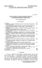
Relative Price Levels
The ratio of the UVR to the exchange rate indicates whether the prices of Brazil and Mexico were
above or under those of the USA. The 1985 and 1988 price levels were extrapolated with trends in
manufacturing prices and nominal exchange rates, see Figure 3. It turns out that Brazilian and
Mexican relative price levels were rather similar between 1970 and 1990. The trends reflects major
changes in exchange rate regimes, such as the decline of the Mexican relative price level after it
dropped its parity with the Dollar in 1976 and depreciated its currency. The trends for Mexico also
show the major devaluations following economic crises such as the debt crisis in 1982 and the peso
crisis at the end of 1994.
17

As Mexico, Brazil tried to maintain a constant exchange rate in the 1970s (it only adopted
mini-devaluations), which together with a relatively high rate of inflation led to an increase of the
price level. A major devaluation (by 30 per cent) did not occur until the end of 1979 explaining the
fall in the relative price level. The contagion of the debt crisis in 1982 led to a major depreciation and
fall in price level. From 1985 onwards, the government maintained the nominal exchange rate while
inflation accelerated, causing a steep rise in the price level. This policy changed in 1989, with a range
of stop-and-go policies, fixing the exchange rate for some months and introducing subsequently major
devaluations. This led to a sharp drop in the price level between 1989 and 1991. In the subsequent
years, the exchange rate was stabilised using massive market interventions, until the introduction of
the Real in July 1994.
Figure 3 also shows the price level of the total economy. In Mexico, the overall price level
was below that of manufacturing during the entire period, as expected by the Balassa Hypothesis. The
trends for manufacturing and the total economy were almost the same. The few years for which PPPs
are available for Brazil show the contrary. This is explained by the introduction of the Real in 1993-
94, which led to a strong increase in the relative price level. Internationally exposed sectors, such as
manufacturing, limited much more than the other sectors the price increases to reduce the loss of
market shares on their home and foreign markets.
Figure 3
Trends in Brazilian and Relative Mexican Price Levels in Manufacturing and
the Total economy, USA =1,00
Brazil
Mexico
1,10
1,1
1,00
0,90
1
0,9
Ratio of RVU to
exchange rate
0,80
0,70
0,60
0,50
Ratio of RVU to
exchange rate
Ratio of PPP to
exchange rate
0,8
0,7
0,6
0,5
Ratio of PPP to
exchange rate
0,40
0,4
0,30
1970 1975 1980 1985 1990 1995
0,3
1970 1975 1980 1985 1990 1995
Sources: benchmark UVRs from Tables 3 and 4, extrapolated with time series of manufacturing deflators derived
by dividing current value added by constant value added from the national accounts as described in Figure 1. PPPs
are from World Bank, World Development Indicators 2001. The price levels of the total economy is measured by
the ratio of the PPP to exchange rate; that of manufacturing is measured by the ratio of the RVU to exchange rate.
Series of nominal exchange rates from CEPII, the CHELEM database.
Productivity Levels
The benchmark estimates for 1985 and 1988 can be extrapolated with time series for value added at
constant prices and employment for the 1970-99 period, see Figure 3. As shown in Figure 2,
productivity growth has been faster in the USA than in Brazil and Mexico. As a consequence, the
productivity gaps between Brazil and Mexico on the one hand and the USA on the other widened over
time. The largest drop in overall relative productivity of the Latin countries occurred in particular
18

during the "lost decade" of the 1980s. In the 1990s, Brazil managed to stabilise the productivity gap,
whereas Mexico's position further eroded after the peso crisis at the end of 1994. As productivity
growth in the USA accelerated in the 1990s, the performance of Mexico until 1995 and that of Brazil
throughout the decade are rather remarkable.
Figure 4
Trends in Labour Productivity Levels,
Brazil/USA and Mexico/USA, 1970-1998 (USA=100)
Brazil/USA
Mexico/USA
120
120
Textiles
100
Machinery
Transport
100
80
80
60
Food
Other
60
Transport
Metals
Textiles
40
20
Chemicals
Wood, Paper
Total
40
20
Wood, Paper
Machinery
Metals
Food
Chemicals
Total
Other
0
1970 1975 1980 1985 1990 1995
0
1970 1975 1980 1985 1990 1995
Sources: benchmark productivity levels from Tables 3 and 4, extrapolated with time series of value added and
employment as described in Figure 1.
The overall trends hide large differences in gains and losses across the different sectors. In
Brazil, most industries lost ground vis-a-vis the USA, except for transport equipment, wood and paper
and to a lesser extent food, beverages and tobacco. For Brazil, consistent series of value added and
employment only exist for the 1990s. These had to be combined with two other series for the 1980s
and the 1970s. In particular for textiles and clothing, machinery and equipment, and transport
equipment, the final series produce odd results in terms of trends in relative productivity levels 6
In Mexico, the only branches that did NOT loose ground relative to their counterparts in the USA are
basic metals and metal products and wood and wood products. As in Brazil, the largest relative
6 For textiles, the Brazilian series show a fall in absolute productivity levels between 1970s and the 1990s,
whereas in according to the US series important productivity gains were achieved in this sector. The
combination of the two trends results in relative productive levels above 100 per cent in the early 1970s.
Another explanation for the high relative level of Brazil in textiles is that the 1985 relative productivity level is
probably overestimated due to the exclusion of non-census establishments, which had much lower productivity.
For transport equipment, the Brazilian series show a substantial cut in employment with continuous positive
output growth resulting in a very high rate of productivity growth in the 1990s. Combined with a moderate rate
of productivity growth in the USA, the relative productivity level of Brazil exceeded 100 per cent after 1995.
19

productivity decline was observed in textiles and clothing. The Mexican time series produce more
plausible results than those of Mexico, partly because of the availability of long run time series of the
national accounts for value added and employment.
An important question is whether the differences in growth rates between Brazil and the USA
in textiles and clothing, machinery and transport equipment are real or due to inconsistencies in the
time series. For this purpose it is useful to check the plausibility of the time series by using them to
backdate our 1985 benchmark estimates to 1975, which is the year for which the first benchmark
comparison was made between Brazil and the USA by van Ark and Maddison (1994). 7 The
extrapolated productivity result from 1985 to 1975 was 56 per cent of the US level, which was 7.5
percentage points higher than the result of Maddison and van Ark. Although the results for food
products and basic metals and metal products were close, those for the other branches show major
discrepancies. This seriously questions the validity of the Brazilian time series.
Table 7
Extrapolation of Relative Productivity Levels to 1975 and
Comparison with Results of van Ark and Maddison (USA=100)
Brazil
Mexico
1985 1975 1988 1975
Extrapolated van Ark and Extrapolated van Ark and
Maddison
Maddison
Food, Beverages and Tobacco 43.9 52.5 56.6 25.5 33.9 36.1
Textiles and Clothing 52.7 100.6 52.5 33.4 60.5 38.2
Wood, Paper and Publishing 28.3 16.2 28.6 22.3 22.5 22.3
Chemicals 32.6 39.2 66.6 31.0 40.0 39.3
Basic Metal and Metal Products 50.8 47.5 42.4 29.4 35.4 42.8
Machinery, Equipment (except Transport) 55.3 99.8 17.5 22.8
51.6
Transport Equipment 55.9 72.2
50.8 69.8
31.3
Other manufacturing 41.3 80.8 39.0 18.9 42.6 29.2
Total Manufacturing 42.5 56.0 48.5 27.4 37.6 37.1
Sources: benchmark results from Table 6, extrapolations based on time series as described in Figure 1.
The same exercise was carried out for the Mexico/USA comparison, see the right hand side of the table. In contrast
to the Brazil/USA comparison, the extrapolated results for Mexico from 1988 to 1975 are very close to those of van
Ark and Maddison. This finding holds for total manufacturing, as well as most branches except textiles and
clothing and other manufacturing.
8. Unit Labour costs
Relative productivity levels are an important determinant of international competitiveness. However,
some countries may not be handicapped by low productivity if at the same time labour compensation
is also low. The net result of relative productivity and relative remuneration is expressed by the
concept of unit labour costs. It divides the labour compensation in Brazil or Mexico relative to the
USA by the labour productivity in Brazil or Mexico relative to the USA:
ULC
( W N )
x
⎛ ⎞
⎜
P
⎝ NER ⎟⎟ P $ ⎠
( W N )
USA
xu $
=
RLPE
(18)
7 It should be stressed that even with exactly the same sources, extrapolated estimates will never exactly compare
with benchmark results for the corresponding year, because of inconsistencies in index numbers.
20

where ULC are unit labour costs, W/N compensation per employee, NER nominal exchange rate,
RLPE relative level of labour productivity, subscripts and superscripts represent x Brazil of Mexico, P
currency of Brazil or Mexico, USA United States and $ dollar. Labour costs of Brazil of Mexico are
expressed in US$ using the exchange rate, as this is the rate used in international transactions. Labour
productivity of the Latin countries, however, is converted into US$ by the UVR as this is the
conversion factor applied to produced output.
Table 8 shows the results for both bilateral comparisons. In Brazil and Mexico, the relatively
low productivity levels are largely compensated by even lower levels of labour compensation: in
Brazil unit labour costs were only 23 per cent of the US level in 1985 and in Mexico only 37 per cent
of the US level. The lowest unit labour costs in Brazil are in furniture and fixtures and food products,
and in Mexico in rubber and plastics and fabricated metal products.
21

Table 8
Relative levels of unit labour costs
Brazil/United States (1985) et Mexico/USA (1988)
SIC Brazil/USA. 1985 Mexico/USA. 1988
Units labour Compensation Labour Units labour Compensation Labour
costs per employee Productivity costs per employee Productivity
(USA=100)
(USA=100)
20 Food products 16.8 7.8 46.5 35.4 9.4 26.5
21 Tobacco Products 41.8 8.6 20.5 35.0 9.3 26.7
22 Textile Mill Products 20.8 11.3 54.4 42.1 15.1 35.8
23 Clothing and apparel 18.0 9.6 53.2 34.7 10.2 29.4
24 Lumber and Wood Products 17.6 6.4 36.5 46.4 6.5 14.0
25 Furniture and Fixtures 11.4 8.2 72.0 53.2 7.5 14.0
26 Paper and Allied Products 24.7 10.5 42.6 48.2 12.7 26.3
27 Printing and Publishing 84.4 11.4 13.5 28.3 9.3 32.9
28 Chemicals and Allied Products 32.6 12.2 37.3 48.3 13.6 28.1
30 Rubber and Plastic Products 38.0 11.8 31.2 11.4 6.2 54.7
31 Leather and Leather Products 18.9 9.3 49.4 31.2 6.8 21.9
32 Stone. Clay. Glass and Concrete Products 21.0 6.5 31.0 55.5 17.8 32.0
33 Primary Metal Industries 61.0 17.8 29.1
22.0 11.2 50.8
34 Fabricated Metal Products
23.8 6.6 27.8
35 Machinery and Computer equipment 17.4 13.2 75.8 56.4 11.6 20.6
36 Electronic and Other Electrical Equipment 34.4 12.5 36.4 59.6 9.4 15.8
37 Transportation Equipment 19.7 11.0 55.9 32.5 16.5 50.8
38 Medical. precision and Optical equipment 13.4 10.1 75.1 73.1 9.2 12.5
39 Miscellaneous Manufacturing Industries 25.1 10.4 41.3 36.1 6.8 18.9
20-39 Total Manufacturing 22.7 9.6 42.5 36.7 10.1 27.4
Sources: relative productivity levels from Table 6 , labour compensation from censuses of manufacturing as
described in Text.
9. Conclusion
International comparisons of productivity levels by industry of origin are a key measure of economic
performance next to comparisons of per capita income and other aggregates measures at the economywide
level. This study assesses the labour productivity gap between Brazil and Mexico on the one
hand and the USA on the other in the mid-1980s. It is an update of Maddison and van Ark (1994),
who assessed the relative performances of these countries in 1975. The paper adopts the ICOP
industry-of-origin methodology developed by the University of Groningen and refined in collaboration
with CEPII. This method uses relative producer prices, also referred to as unit value ratios (UVRs)
instead of exchange rates or proxy PPPs to express the output of different countries in a common
currency (here US$). The paper introduced reliability tests for the UVRs using coefficient of
variation. It turned out that both the UVRs of both Brazil/USA and Mexico/USA are well within the
confidence intervals, although the variation of the former are higher than that of the latter bilateral
comparison. Moreover, the representativeness of the Mexico/USA comparison is far greater than that
of the Brazil/USA comparisons, as the relative price estimates are based on a substantially larger part
of output in the latter comparison.
Brazilian productivity in 1985 was 42.5 per cent of the US level and that of Mexico in 1988
27.4 per cent. Large variations across sectors exist with regard to relative productivity levels. The
reliability tests of the UVRs indicate that in some branches our measures need to be improved, either
with new product matches or quality adjustments. However, the most problematic issue, which falls
outside the immediate scope of the ICOP methodology, concerns the Brazilian time series of value
added and employment used to extrapolate our benchmark results for the 1970-99 period. In particular
22

the time series for textiles and clothing, and machinery and transport equipment seem very
implausible. An alternative and probably more reliable method is to redo a full benchmark
comparison each decade. As such the ICOP estimates of comparative labour productivity in textiles
and clothing, wood, paper and publishing, machinery and transport equipment and other
manufacturing between the 1975 and the 1985 benchmark estimates seem much more plausible than
the huge relative productivity changes suggested by the backward extrapolation procedure (see Table
8). To obtain reliable results the 1990s, the way forward therefore also seems to carry out a new set of
bilateral comparisons instead of relying on the extrapolated results from 1985 and 1988.
Another area which requires further investigation is the reliability of the national accounts of
Brazil and Mexico, and in particular the practice of both countries in estimating value added of
informal activity. The Mexican accounts add more than a third to the census estimate of value added,
whereas the Brazilians do not seem to make any imputation, in spite of evidence from employment
statistics that informal activity is proportionally comparable between the two countries. Van Ark and
Maddison (1994) already observed this for 1975, and it would be interesting to check this with the new
evidence for the 1990s.
In order to understand the differences in economics performances between Brazil and Mexico,
the analysis can be extended with new variables. In particular, it would be interesting to compare the
investment behaviour between the two countries, and as such the contribution of capital to labour
productivity differences. Hofman and Mulder (1998) presented some rough comparative estimates of
labour, capital and multi-factor productivity in manufacturing in Brazil and Mexico. These results
could be refined, although sectoral investment data, necessary to build capital stocks, in Brazil and
Mexico have to be used with great care. Other variables that would greatly contribute to the
understanding of manufacturing performance include human capital, and institutional factors that
account for differences in the pace of economic and international trade reforms in both countries in the
1980s and 1990s.
23

References
Ark, B. van and A Maddison (1994), “An International Comparison of Real Output, Purchasing Power
and Labour Productivity in Manufacturing Industries: Brazil, Mexico and the USA in 1975”,
Research Memorandum, No. 567 (GD-6), Groningen Growth and Development Centre.
Ark, B. van , R. Inklaar and M. Timmer (2000), “The Canada-US Manufacturing of Productivity Gap
revisited: new ICOP Results”, paper presented at the CSLS Conference on the Canada-US
Manufacturing Productivity Gap, January 21-22
Ark. B. van and M. Timmer (2001) "PPPs and International Productivity Comparisons: Bottlenecks
and New Directions", paper presented Joint World Bank/OECD seminar on purchasing power
parities, 30 January – 2 February, Washington DC.
Chevallier, A. and D. Unal-Kesenci (2001), “La productivité des industries méditerranéennes”,
Working Paper, CEPII, Paris, forthcoming.
Cottenet H. & N. Mulder (2001), “The Competitiveness of Egyptian Manufacturing: An International
Perspective”, Working Paper, CEPII, Paris, forthcoming.
Freudenberg, M. and D. Unal-Kesenci, 1994. “French and German Productivity Levels in
Manufacturing”, Working Paper, No. 94-10, CEPII, Paris.
Hofman, A. and N. Mulder (1998), “The Comparative Productivity Performance of Brazil and
Mexico, 1950-94”, with in J. Coatsworth and A. Taylor (eds.), Latin America and the World
Economy in the Nineteenth and Twentieth Centuries: Explorations in Quantitative Economic
History, Harvard University Press.
Kravis, I.B., A. Heston and R. Summers (1982), World Product and Income: International
Comparisons of Real Gross Product, Johns Hopkins University Press, Baltimore.
Mulder, N., L. Peres and S. Montout (2001), “Brazil and Mexico's Comparative Manufacturing
Performance in the 1980s”, Working Paper, CEPII, Paris, forthcoming.
Nayman L. & D. Ünal-Kesenci (2001), “The France-Germany Manufacturing Productivity
Comparison: Ten Years After the German Reunification”, Working Paper, CEPII, Paris,
forthcoming.
Paige, D. and G. Bombach (1959), A Comparison of National Output and Productivity of the United
Kingdom and the United States, OEEC and the University of Cambridge, Paris.
Rostas, L. (1948), Comparative Productivity in British and American Industries, NIESR, Occasional
Papers, No. 13, Cambridge University Press, Cambridge.
Selvanathan (1991),
Timmer, M., B. van Ark, N. Mulder, L. Nayman and D.Ünal-Kesenci (2001), "Formalization of the
ICOP methodology for binary manufacturing comparisons", mimeo, University of Groningen
and CEPII, Groningen and Paris.
24

Papers issued in the series of the Groningen Growth and Development Centre
Papers marked * are also available in pdf-format on the internet: http://www.eco.rug.nl/ggdc/
536 (GD-1) Maddison, Angus and Harry van Ooststroom, The International Comparison of Value
Added, Productivity and Purchasing Power Parities in Agriculture (1993)
537 (GD-2) Mulder, Nanno and Angus Maddison, The International Comparison of Performance in
Distribution: Value Added, Labour Productivity and PPPs in Mexican and US Wholesale
and Retail Trade 1975/7 (1993)
538 (GD-3) Szirmai, Adam, Comparative Performance in Indonesian Manufacturing, 1975-90 (1993)
549 (GD-4) de Jong, Herman J., Prices, Real Value Added and Productivity in Dutch Manufacturing,
1921-1960 (1993)
550 (GD-5) Beintema, Nienke and Bart van Ark, Comparative Productivity in East and West German
Manufacturing before Reunification (1993)
567 (GD-6) Maddison, Angus and Bart van Ark, The International Comparison of Real Product and
Productivity (1994)
568 (GD-7) de Jong, Gjalt, An International Comparison of Real Output and Labour Productivity in
Manufacturing in Ecuador and the United States, 1980 (1994)
569 (GD-8) van Ark, Bart and Angus Maddison, An International Comparison of Real Output,
Purchasing Power and Labour Productivity in Manufacturing Industries: Brazil, Mexico
and the USA in 1975 (1994) (second edition)
570 (GD-9) Maddison, Angus, Standardised Estimates of Fixed Capital Stock: A Six Country
Comparison (1994)
571 (GD-10) van Ark, Bart and Remco D.J. Kouwenhoven, Productivity in French Manufacturing: An
International Comparative Perspective (1994)
572 (GD-11) Gersbach, Hans and Bart van Ark, Micro Foundations for International Productivity
Comparisons (1994)
573 (GD-12) Albers, Ronald, Adrian Clemens and Peter Groote, Can Growth Theory Contribute to
Our Understanding of Nineteenth Century Economic Dynamics (1994)
574 (GD-13) de Jong, Herman J. and Ronald Albers, Industrial Output and Labour Productivity in the
Netherlands, 1913-1929: Some Neglected Issues (1994)
575 (GD-14) Mulder, Nanno, New Perspectives on Service Output and Productivity: A Comparison of
French and US Productivity in Transport, Communications Wholesale and Retail Trade
(1994)
576 (GD-15) Maddison, Angus, Economic Growth and Standards of Living in the Twentieth Century
(1994)
577 (GD-16) Gales, Ben, In Foreign Parts: Free-Standing Companies in the Netherlands around the
First World War (1994)
578 (GD-17) Mulder, Nanno, Output and Productivity in Brazilian Distribution: A Comparative View
(1994)
579 (GD-18) Mulder, Nanno, Transport and Communication in Mexico and the United States: Value
Added, Purchasing Power Parities and Productivity (1994)
25

580 (GD-19) Mulder, Nanno, Transport and Communications Output and Productivity in Brazil and
the USA, 1950-1990 (1995)
581 (GD-20) Szirmai, Adam and Ren Ruoen, China's Manufacturing Performance in Comparative
Perspective, 1980-1992 (1995)
GD-21 Fremdling, Rainer, Anglo-German Rivalry on Coal Markets in France, the Netherlands
and Germany, 1850-1913 (December 1995)
GD-22 Tassenaar, Vincent, Regional Differences in Standard of Living in the Netherlands,
1800-1875. A Study Based on Anthropometric Data (December 1995)
GD-23 van Ark, Bart, Sectoral Growth Accounting and Structural Change in Postwar Europe
(December 1995)
GD-24 Groote, Peter, Jan Jacobs and Jan Egbert Sturm, Output Responses to Infrastructure in the
Netherlands, 1850-1913 (December 1995)
GD-25 Groote, Peter, Ronald Albers and Herman de Jong, A Standardised Time Series of the
Stock of Fixed Capital in the Netherlands, 1900-1995 (May 1996)
GD-26 van Ark, Bart and Herman de Jong, Accounting for Economic Growth in the Netherlands
since 1913 (May 1996)
GD-27* Maddison, Angus and D.S. Prasada Rao, A Generalized Approach to International
Comparisons of Agricultural Output and Productivity (May 1996)
GD-28 van Ark, Bart, Issues in Measurement and International Comparison of Productivity - An
Overview (May 1996)
GD-29* Kouwenhoven, Remco, A Comparison of Soviet and US Industrial Performance, 1928-
90 (May 1996)
GD-30 Fremdling, Rainer, Industrial Revolution and Scientific and Technological Progress
(December 1996)
GD-31 Timmer, Marcel, On the Reliability of Unit Value Ratios in International Comparisons
(December 1996)
GD-32 de Jong, Gjalt, Canada's Post-War Manufacturing Performance: A Comparison with the
United States (December 1996)
GD-33 Lindlar, Ludger, “1968” and the German Economy (January 1997)
GD-34 Albers, Ronald, Human Capital and Economic Growth: Operationalising Growth Theory,
with Special Reference to The Netherlands in the 19th Century (June 1997)
GD-35 Brinkman, Henk-Jan, J.W. Drukker and Brigitte Slot, GDP per Capita and the Biological
Standard of Living in Contemporary Developing Countries (June 1997)
GD-36 de Jong, Herman, and Antoon Soete, Comparative Productivity and Structural Change in
Belgian and Dutch Manufacturing, 1937-1987 (June 1997)
GD-37 Timmer, M.P., and A. Szirmai, Growth and Divergence in Manufacturing Performance in
South and East Asia (June 1997)
GD-38* van Ark, B., and J. de Haan, The Delta-Model Revisited: Recent Trends in the
GD-39*
GD-40*
Structural Performance of the Dutch Economy (December 1997)
van der Eng, P., Economics Benefits from Colonial Assets: The Case of the
Netherlands and Indonesia, 1870-1958 (June 1998)
Timmer, Marcel P., Catch Up Patterns in Newly Industrializing Countries. An
International Comparison of Manufacturing Productivity in Taiwan, 1961-1993 (July
1998)
26

GD-41*
van Ark, Bart, Economic Growth and Labour Productivity in Europe: Half a Century of
East-West Comparisons (October 1999)
GD-42* Smits, Jan Pieter, Herman de Jong and Bart van Ark, Three Phases of Dutch Economic
Growth and Technological Change, 1815-1997 (October 1999)
GD-43* Fremdling, Rainer, Historical Precedents of Global Markets (October 1999)
GD-44* van Ark, Bart, Lourens Broersma and Gjalt de Jong, Innovation in Services. Overview of
Data Sources and Analytical Structures (October 1999)
GD-45* Broersma, Lourens and Robert McGuckin, The Impact of Computers on Productivity in
the Trade Sector: Explorations with Dutch Microdata (October 1999, Revised version
June 2000)
GD-46* Sleifer, Jaap, Separated Unity: The East and West German Industrial Sector in 1936
(November 1999)
GD-47* Rao, D.S. Prasada and Marcel Timmer, Multilateralisation of Manufacturing Sector
Comparisons: Issues, Methods and Empirical Results (July 2000)
GD-48* Vikström, Peter, Long term Patterns in Swedish Growth and Structural Change, 1870-
1990 (July 2001)
GD-49* Wu, Harry X., Comparative labour productivity performance in Chinese manufacturing,
1952-1997: An ICOP PPP Approach (July 2001)
GD-50* Monnikhof, Erik and Bart van Ark, New Estimates of Labour Productivity in the
Manufacturing sectors of Czech Republic, Hungary and Poland, 1996 (January 2002)
GD-51* van Ark, Bart, Robert Inklaar and Marcel Timmer, The Canada-US Manufacturing Gap
Revisited: New ICOP Results (January 2002)
GD-52* Mulder, Nanno, Sylvie Montout and Luis Peres Lopes, Brazil and Mexico's
Manufacturing Performance in International Perspective, 1970-98 (January 2002)
Groningen Growth and Development Centre Research Monographs:
Monographs marked * are also available in pdf-format on the internet
No. 1* van Ark, Bart, International Comparisons of Output and Productivity: Manufacturing
Productivity Performance of Ten Countries from 1950 to 1990 (1993)
(http://www.eco.rug.nl/GGDC/pub/Arkbook.shtml)
No. 2 Pilat, Dirk, The Economics of Catch-Up: The Experience of Japan and Korea (1993)
No. 3
No. 4
No. 5*
Hofman, André, Latin American Economic Development. A Causal Analysis in
Historical Perspective (1998)
Mulder, Nanno, The Economic Performance of the Service Sector in Brazil, Mexico and
the United States (1999)
Smits, Jan-Pieter, Edwin Horlings and Jan Luiten van Zanden, Dutch
GNP and Its Components, 1800-1913 (2000)
(http://www.eco.rug.nl/GGDC/PUB/dutchgnp.pdf)
27