Chapter 5 - Analytical Sciences Digital Library

Chapter 5
Standardizing Analytical
Chapter Overview
Methods
5A Analytical Standards
5B Calibrating the Signal (S total )
5C Determining the Sensitivity (k A )
5D Linear Regression and Calibration Curves
5E Compensating for the Reagent Blank (S reag )
5F Using Excel and R for a Regression Analysis
5G Key Terms
5H Chapter Summary
5I Problems
5J Solutions to Practice Exercises
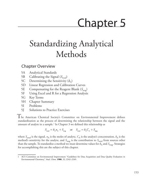
The American Chemical Society’s Committee on Environmental Improvement defines
standardization as the process of determining the relationship between the signal and the
amount of analyte in a sample. 1 In Chapter 3 we defined this relationship as
S = k n + S or S = k C + S
total A A reag total A A r eag
where S total is the signal, n A is the moles of analyte, C A is the analyte’s concentration, k A is the
method’s sensitivity for the analyte, and S reag is the contribution to S total from sources other
than the sample. To standardize a method we must determine values for k A and S reag . Strategies
for accomplishing this are the subject of this chapter.
1 ACS Committee on Environmental Improvement “Guidelines for Data Acquisition and Data Quality Evaluation in
Environmental Chemistry,” Anal. Chem. 1980, 52, 2242–2249.
153

154 Analytical Chemistry 2.0
See Chapter 9 for a thorough discussion of
titrimetric methods of analysis.
The base NaOH is an example of a secondary
standard. Commercially available
NaOH contains impurities of NaCl,
Na 2 CO 3 , and Na 2 SO 4 , and readily
absorbs H 2 O from the atmosphere. To
determine the concentration of NaOH in
a solution, it is titrated against a primary
standard weak acid, such as potassium hydrogen
phthalate, KHC 8 H 4 O 4 .
5A
Analytical Standards
To standardize an analytical method we use standards containing known
amounts of analyte. The accuracy of a standardization, therefore, depends
on the quality of the reagents and glassware used to prepare these standards.
For example, in an acid–base titration the stoichiometry of the acid–base reaction
defines the relationship between the moles of analyte and the moles
of titrant. In turn, the moles of titrant is the product of the titrant’s concentration
and the volume of titrant needed to reach the equivalence point.
The accuracy of a titrimetric analysis, therefore, can be no better than the
accuracy to which we know the titrant’s concentration.
5A.1 Primary and Secondary Standards
We divide analytical standards into two categories: primary standards and
secondary standards. A primary standard is a reagent for which we can
dispense an accurately known amount of analyte. For example, a 0.1250-g
sample of K 2 Cr 2 O 7 contains 4.249 × 10 –4 moles of K 2 Cr 2 O 7 . If we place
this sample in a 250-mL volumetric flask and dilute to volume, the concentration
of the resulting solution is 1.700 × 10 –3 M. A primary standard
must have a known stoichiometry, a known purity (or assay), and it must
be stable during long-term storage. Because of the difficulty in establishing
the degree of hydration, even after drying, a hydrated reagent usually is not
a primary standard.
Reagents that do not meet these criteria are secondary standards.
The concentration of a secondary standard must be determined relative
to a primary standard. Lists of acceptable primary standards are available. 2
Appendix 8 provides examples of some common primary standards.
5A.2 Other Reagents
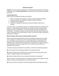
Preparing a standard often requires additional reagents that are not primary
standards or secondary standards. Preparing a standard solution, for
example, requires a suitable solvent, and additional reagents may be need
to adjust the standard’s matrix. These solvents and reagents are potential
sources of additional analyte, which, if not accounted for, produce a determinate
error in the standardization. If available, reagent grade chemicals
conforming to standards set by the American Chemical Society should be
used. 3 The label on the bottle of a reagent grade chemical (Figure 5.1) lists
either the limits for specific impurities, or provides an assay for the impurities.
We can improve the quality of a reagent grade chemical by purifying it,
or by conducting a more accurate assay. As discussed later in the chapter, we
2 (a) Smith, B. W.; Parsons, M. L. J. Chem. Educ. 1973, 50, 679–681; (b) Moody, J. R.; Greenburg,
P. R.; Pratt, K. W.; Rains, T. C. Anal. Chem. 1988, 60, 1203A–1218A.
3 Committee on Analytical Reagents, Reagent Chemicals, 8th ed., American Chemical Society:
Washington, D. C., 1993.

Chapter 5 Standardizing Analytical Methods
155
can correct for contributions to S total from reagents used in an analysis by
including an appropriate blank determination in the analytical procedure.
5A.3 Preparing Standard Solutions
It is often necessary to prepare a series of standards, each with a different
concentration of analyte. We can prepare these standards in two ways. If the
range of concentrations is limited to one or two orders of magnitude, then
each solution is best prepared by transferring a known mass or volume of
the pure standard to a volumetric flask and diluting to volume.
When working with larger ranges of concentration, particularly those
extending over more than three orders of magnitude, standards are best prepared
by a serial dilution from a single stock solution. In a serial dilution
we prepare the most concentrated standard and then dilute a portion of it
to prepare the next most concentrated standard. Next, we dilute a portion
of the second standard to prepare a third standard, continuing this process
until all we have prepared all of our standards. Serial dilutions must be prepared
with extra care because an error in preparing one standard is passed
on to all succeeding standards.
(a)
(b)
Figure 5.1 Examples of typical packaging labels for reagent grade chemicals. Label
(a) provides the manufacturer’s assay for the reagent, NaBr. Note that potassium
is flagged with an asterisk (*) because its assay exceeds the limits established by
the American Chemical Society (ACS). Label (b) does not provide an assay for
impurities, but indicates that the reagent meets ACS specifications. An assay for
the reagent, NaHCO 3 is provided.

156 Analytical Chemistry 2.0
See Section 2D.1 to review how an electronic
balance works. Calibrating a balance
is important, but it does not eliminate all
sources of determinate error in measuring
mass. See Appendix 9 for a discussion of
correcting for the buoyancy of air.
5B Calibrating the Signal (S total )
The accuracy of our determination of k A and S reag depends on how accurately
we can measure the signal, S total . We measure signals using equipment, such
as glassware and balances, and instrumentation, such as spectrophotometers
and pH meters. To minimize determinate errors affecting the signal,
we first calibrate our equipment and instrumentation. We accomplish the
calibration by measuring S total for a standard with a known response of S std ,
adjusting S total until
S
total
= S
Here are two examples of how we calibrate signals. Other examples are
provided in later chapters focusing on specific analytical methods.
When the signal is a measurement of mass, we determine S total using
an analytical balance. To calibrate the balance’s signal we use a reference
weight that meets standards established by a governing agency, such as the
National Institute for Standards and Technology or the American Society
for Testing and Materials. An electronic balance often includes an internal
calibration weight for routine calibrations, as well as programs for calibrating
with external weights. In either case, the balance automatically adjusts
S total to match S std .
We also must calibrate our instruments. For example, we can evaluate
a spectrophotometer’s accuracy by measuring the absorbance of a carefully
prepared solution of 60.06 mg/L K 2 Cr 2 O 7 in 0.0050 M H 2 SO 4 , using
0.0050 M H 2 SO 4 as a reagent blank. 4 An absorbance of 0.640 ± 0.010
absorbance units at a wavelength of 350.0 nm indicates that the spectrometer’s
signal is properly calibrated. Be sure to read and carefully follow the
calibration instructions provided with any instrument you use.
std
5C Determining the Sensitivity (k A )
To standardize an analytical method we also must determine the value of
k A in equation 5.1 or equation 5.2.
S = k n + S
total A A reag
5.1
S = k C + S
total A A reag
5.2
In principle, it should be possible to derive the value of k A for any analytical
method by considering the chemical and physical processes generating
the signal. Unfortunately, such calculations are not feasible when we lack
a sufficiently developed theoretical model of the physical processes, or are
not useful because of nonideal chemical behavior. In such situations we
must determine the value of k A by analyzing one or more standard solutions,
each containing a known amount of analyte. In this section we consider
4 Ebel, S. Fresenius J. Anal. Chem. 1992, 342, 769.

Chapter 5 Standardizing Analytical Methods
157
several approaches for determining the value of k A . For simplicity we will
assume that S reag has been accounted for by a proper reagent blank, allowing
us to replace S total in equation 5.1 and equation 5.2 with the analyte’s
signal, S A .
S
S
= k n
5.3
A A A
= k C
5.4
A A A
5C.1 Single-Point versus Multiple-Point Standardizations
The simplest way to determine the value of k A in equation 5.4 is by a single-point
standardization in which we measure the signal for a standard,
S std , containing a known concentration of analyte, C std . Substituting these
values into equation 5.4
k
A
Sstd
= 5.5
C
gives the value for k A . Having determined the value for k A , we can calculate
the concentration of analyte in any sample by measuring its signal, S samp ,
and calculating C A using equation 5.6.
C
A
std
Ssamp
= 5.6
k
A single-point standardization is the least desirable method for standardizing
a method. There are at least two reasons for this. First, any error
in our determination of k A carries over into our calculation of C A . Second,
our experimental value for k A is for a single concentration of analyte. Extending
this value of k A to other concentrations of analyte requires us to
assume a linear relationship between the signal and the analyte’s concentration,
an assumption that often is not true. 5 Figure 5.2 shows how assuming
a constant value of k A may lead to a determinate error in the analyte’s
concentration. Despite these limitations, single-point standardizations find
routine use when the expected range for the analyte’s concentrations is
small. Under these conditions it is often safe to assume that k A is constant
(although you should verify this assumption experimentally). This is the
case, for example, in clinical labs where many automated analyzers use only
a single standard.
The preferred approach to standardizing a method is to prepare a series
of standards, each containing the analyte at a different concentration.
Standards are chosen such that they bracket the expected range for the analyte’s
concentration. A multiple-point standardization should include
at least three standards, although more are preferable. A plot of S std versus
A
Equation 5.3 and equation 5.4 are essentially
identical, differing only in whether
we choose to express the amount of analyte
in moles or as a concentration. For the
remainder of this chapter we will limit our
treatment to equation 5.4. You can extend
this treatment to equation 5.3 by replacing
C A with n A .
Linear regression, which also is known as
the method of least squares, is one such algorithm.
Its use is covered in Section 5D.
5 Cardone, M. J.; Palmero, P. J.; Sybrandt, L. B. Anal. Chem. 1980, 52, 1187–1191.

158 Analytical Chemistry 2.0
assumed relationship
actual relationship
S samp
Figure 5.2 Example showing how a single-point
standardization leads to a determinate error in an
analyte’s reported concentration if we incorrectly
assume that the value of k A is constant.
S std
C std
(C A ) reported
(C A ) actual
C std is known as a calibration curve. The exact standardization, or calibration
relationship is determined by an appropriate curve-fitting algorithm.
There are at least two advantages to a multiple-point standardization.
First, although a determinate error in one standard introduces a determinate
error into the analysis, its effect is minimized by the remaining standards.
Second, by measuring the signal for several concentrations of analyte we
no longer must assume that the value of k A is independent of the analyte’s
concentration. Constructing a calibration curve similar to the “actual relationship”
in Figure 5.2, is possible.
Appending the adjective “external” to the
noun “standard” might strike you as odd
at this point, as it seems reasonable to assume
that standards and samples must
be analyzed separately. As you will soon
learn, however, we can add standards to
our samples and analyze them simultaneously.
5C.2 External Standards
The most common method of standardization uses one or more external
standards, each containing a known concentration of analyte. We call
them “external” because we prepare and analyze the standards separate from
the samples.
Si n g l e Ex t e r n a l St a n d a r d
A quantitative determination using a single external standard was described
at the beginning of this section, with k A given by equation 5.5. After determining
the value of k A , the concentration of analyte, C A , is calculated
using equation 5.6.
Example 5.1
A spectrophotometric method for the quantitative analysis of Pb 2+ in
blood yields an S std of 0.474 for a single standard whose concentration of
lead is 1.75 ppb What is the concentration of Pb 2+ in a sample of blood
for which S samp is 0.361

Chapter 5 Standardizing Analytical Methods
159
So l u t i o n
Equation 5.5 allows us to calculate the value of k A for this method using
the data for the standard.
k
A
Sstd
0.
474
= = = 0.
2709 ppb
C 175 . ppb
std
Having determined the value of k A , the concentration of Pb 2+ in the sample
of blood is calculated using equation 5.6.
C
A
Ssamp
0.
361
= = = 133 . ppb
-1
k 0.
2709 ppb
A
-1
Mu l t i p l e Ex t e r n a l St a n d a r d s
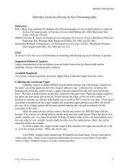
Figure 5.3 shows a typical multiple-point external standardization. The
volumetric flask on the left is a reagent blank and the remaining volumetric
flasks contain increasing concentrations of Cu 2+ . Shown below the
volumetric flasks is the resulting calibration curve. Because this is the most
common method of standardization the resulting relationship is called a
normal calibration curve.
When a calibration curve is a straight-line, as it is in Figure 5.3, the
slope of the line gives the value of k A . This is the most desirable situation
since the method’s sensitivity remains constant throughout the analyte’s
concentration range. When the calibration curve is not a straight-line, the
0.25
0.20
S std
0.15
0.10
0.05
0
0 0.0020 0.0040 0.0060 0.0080
C std
(M)
Figure 5.3 Shown at the top is a reagent
blank (far left) and a set of five external
standards for Cu 2+ with concentrations
increasing from left to right.
Shown below the external standards is
the resulting normal calibration curve.
The absorbance of each standard, S std ,
is shown by the filled circles.

160 Analytical Chemistry 2.0
method’s sensitivity is a function of the analyte’s concentration. In Figure
5.2, for example, the value of k A is greatest when the analyte’s concentration
is small and decreases continuously for higher concentrations of analyte.
The value of k A at any point along the calibration curve in Figure 5.2 is given
by the slope at that point. In either case, the calibration curve provides a
means for relating S samp to the analyte’s concentration.
Example 5.2
A second spectrophotometric method for the quantitative analysis of Pb 2+
in blood has a normal calibration curve for which
S
std
-1
= ( 0. 296 ppb )× C + 0.
003
What is the concentration of Pb 2+ in a sample of blood if S samp is 0.397
So l u t i o n
To determine the concentration of Pb 2+ in the sample of blood we replace
S std in the calibration equation with S samp and solve for C A .
C
A
S −0.
003
samp 0. 397 −0.
003
=
=
= 133 . ppb
-1
-1
0.
296 ppb 0. 296 ppb
It is worth noting that the calibration equation in this problem includes
an extra term that does not appear in equation 5.6. Ideally we expect
the calibration curve to have a signal of zero when C A is zero. This is the
purpose of using a reagent blank to correct the measured signal. The extra
term of +0.003 in our calibration equation results from the uncertainty in
measuring the signal for the reagent blank and the standards.
std
The one-point standardization in this exercise
uses data from the third volumetric
flask in Figure 5.3.
Practice Exercise 5.1
Figure 5.3 shows a normal calibration curve for the quantitative analysis
of Cu 2+ . The equation for the calibration curve is
S std = 29.59 M –1 × C std + 0.0015
What is the concentration of Cu 2+ in a sample whose absorbance, S samp ,
is 0.114 Compare your answer to a one-point standardization where a
standard of 3.16 × 10 –3 M Cu 2+ gives a signal of 0.0931.
Click here to review your answer to this exercise.
An external standardization allows us to analyze a series of samples
using a single calibration curve. This is an important advantage when we
have many samples to analyze. Not surprisingly, many of the most common
quantitative analytical methods use an external standardization.
There is a serious limitation, however, to an external standardization.
When we determine the value of k A using equation 5.5, the analyte is pres-

Chapter 5 Standardizing Analytical Methods
161
S samp
standard’s
matrix
sample’s
matrix
(C A ) reported
(C A ) actual
Figure 5.4 Calibration curves for an analyte in the
standard’s matrix and in the sample’s matrix. If the
matrix affects the value of k A , as is the case here, then
we introduce a determinate error into our analysis if
we use a normal calibration curve.
ent in the external standard’s matrix, which usually is a much simpler matrix
than that of our samples. When using an external standardization we
assume that the matrix does not affect the value of k A . If this is not true,
then we introduce a proportional determinate error into our analysis. This
is not the case in Figure 5.4, for instance, where we show calibration curves
for the analyte in the sample’s matrix and in the standard’s matrix. In this
example, a calibration curve using external standards results in a negative
determinate error. If we expect that matrix effects are important, then we
try to match the standard’s matrix to that of the sample. This is known as
matrix matching. If we are unsure of the sample’s matrix, then we must
show that matrix effects are negligible, or use an alternative method of standardization.
Both approaches are discussed in the following section.
The matrix for the external standards in
Figure 5.3, for example, is dilute ammonia,
which is added because the Cu(NH 3 ) 4
2+
complex absorbs more strongly than
Cu 2+ . If we fail to add the same amount
of ammonia to our samples, then we will
introduce a proportional determinate error
into our analysis.
5C.3 Standard Additions
We can avoid the complication of matching the matrix of the standards to
the matrix of the sample by conducting the standardization in the sample.
This is known as the method of standard additions.
Si n g l e St a n d a r d Ad d i t i o n
The simplest version of a standard addition is shown in Figure 5.5. First we
add a portion of the sample, V o , to a volumetric flask, dilute it to volume,
V f , and measure its signal, S samp . Next, we add a second identical portion
of sample to an equivalent volumetric flask along with a spike, V std , of an
external standard whose concentration is C std . After diluting the spiked
sample to the same final volume, we measure its signal, S spike . The following
two equations relate S samp and S spike to the concentration of analyte, C A , in
the original sample.

162 Analytical Chemistry 2.0
add V o of C A
add V std of C std
Figure 5.5 Illustration showing the method of standard
additions. The volumetric flask on the left contains
a portion of the sample, V o , and the volumetric
flask on the right contains an identical portion of the
sample and a spike, V std , of a standard solution of the
analyte. Both flasks are diluted to the same final volume,
V f . The concentration of analyte in each flask is
shown at the bottom of the figure where C A is the analyte’s
concentration in the original sample and C std is
the concentration of analyte in the external standard.
Concentration
of Analyte
C
A
dilute to V f
Vo
× C
V
f
A
V V
o
× + C ×
std
V V
f
std
f
The ratios V o /V f and V std /V f account for
the dilution of the sample and the standard,
respectively.
S
k C V o
= 5.7
V
samp A A
f
V V
o
std
S k C C
spike
=
Af A
+ V
std
p V 5.8
f
f
As long as V std is small relative to V o , the effect of the standard’s matrix on
the sample’s matrix is insignificant. Under these conditions the value of k A
is the same in equation 5.7 and equation 5.8. Solving both equations for
k A and equating gives
S
samp
C V A
V
o
f
=
C V A
V
o
f
S
spike
+ C
which we can solve for the concentration of analyte, C A , in the original
sample.
Example 5.3
A third spectrophotometric method for the quantitative analysis of Pb 2+ in
blood yields an S samp of 0.193 when a 1.00 mL sample of blood is diluted
to 5.00 mL. A second 1.00 mL sample of blood is spiked with 1.00 mL of
a 1560-ppb Pb 2+ external standard and diluted to 5.00 mL, yielding an
std
V V
std
f
5.9

Chapter 5 Standardizing Analytical Methods
163
S spike of 0.419. What is the concentration of Pb 2+ in the original sample
of blood
So l u t i o n
We begin by making appropriate substitutions into equation 5.9 and solving
for C A . Note that all volumes must be in the same units; thus, we first
covert V std from 1.00 mL to 1.00 × 10 –3 mL.
C
A
0.
193
100 . mL
500 . mL
=
C
A
10 . 0
500 .
mL
mL
0.
419
100 . × 10 −3
mL
+ 1560 ppb
500 . mL
0.
193
0.
419
=
0.
200C
0. 200C
+ 0.
3120 ppb
A A
0.0386C A + 0.0602 ppb = 0.0838C A
0.0452C A = 0.0602 ppb
C A = 1.33 ppb
The concentration of Pb 2+ in the original sample of blood is 1.33 ppb.
It also is possible to make a standard addition directly to the sample,
measuring the signal both before and after the spike (Figure 5.6). In this
case the final volume after the standard addition is V o + V std and equation
5.7, equation 5.8, and equation 5.9 become
add V std of C std
V o
V o
Concentration
of Analyte
C A
C
A
V
o
V
o
+ V
std
+ C
std
V
o
V
std
+ V
std
Figure 5.6 Illustration showing an alternative form of the method of standard additions.
In this case we add a spike of the external standard directly to the sample
without any further adjust in the volume.

164 Analytical Chemistry 2.0
S
= k C
samp A A
V
V
o
std
S k C C
spike
=
Af A
+ V V
std p
+ V + V
5.10
o
std
o
std
S
samp
C
A
=
C
A
V
o
V
o
+ V
std
S
spike
+ C
std
V
o
V
std
+ V
std
5.11
Example 5.4
A fourth spectrophotometric method for the quantitative analysis of Pb 2+
in blood yields an S samp of 0.712 for a 5.00 mL sample of blood. After spiking
the blood sample with 5.00 mL of a 1560-ppb Pb 2+ external standard,
an S spike of 1.546 is measured. What is the concentration of Pb 2+ in the
original sample of blood.
V o + V std = 5.00 mL + 5.00×10 –3 mL
= 5.005 mL
So l u t i o n
To determine the concentration of Pb 2+ in the original sample of blood, we
make appropriate substitutions into equation 5.11 and solve for C A .
0. 712 1.
546
=
3
C
A 500 . mL
500 . × 10
− mL
C
+ 1560
ppb
A
5.
005 mL
5.
005 mL
0. 712 1.
546
=
C 0. 9990C
+ 1.
558 ppb
A A
0.7113C A + 1.109 ppb = 1.546C A
C A = 1.33 ppb
The concentration of Pb 2+ in the original sample of blood is 1.33 ppb.
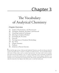
Mu l t i p l e St a n d a r d Ad d i t i o ns
We can adapt the single-point standard addition into a multiple-point
standard addition by preparing a series of samples containing increasing
amounts of the external standard. Figure 5.7 shows two ways to plot a
standard addition calibration curve based on equation 5.8. In Figure 5.7a
we plot S spike against the volume of the spikes, V std . If k A is constant, then
the calibration curve is a straight-line. It is easy to show that the x-intercept
is equivalent to –C A V o /C std .

Chapter 5 Standardizing Analytical Methods
165
(a)
0.60
S spike
6.00
C std
0.50
y-intercept = k AC A V o
V f
0.40
0.30
slope = k AC std
V f
0.20
0.10
0
-2.00 0 2.00 4.00
V std
x-intercept = -C (mL)
AV o
C std
(b)
S spike
0.60
0.50
0.40
0.30
y-intercept = k AC A V o
V f
slope = k A
0.20
0.10
0
-4.00 -2.00 0 2.00 4.00 6.00 8.00 10.00 12.00
V std
x-intercept = -C AV o
V f
×
Vf
(mg/L)
Figure 5.7 Shown at the top is a set of
six standard additions for the determination
of Mn 2+ . The flask on the left
is a 25.00 mL sample diluted to 50.00
mL. The remaining flasks contain 25.00
mL of sample and, from left to right,
1.00, 2.00, 3.00, 4.00, and 5.00 mL
of an external standard of 100.6 mg/L
Mn 2+ . Shown below are two ways to
plot the standard additions calibration
curve. The absorbance for each standard
addition, S spike , is shown by the
filled circles.
Example 5.5
Beginning with equation 5.8 show that the equations in Figure 5.7a for
the slope, the y-intercept, and the x-intercept are correct.
So l u t i o n
We begin by rewriting equation 5.8 as
S
spike
kCV kC
A A o A std
= + × V
V V
which is in the form of the equation for a straight-line
f
Y = y-intercept + slope × X
f
std

166 Analytical Chemistry 2.0
where Y is S spike and X is V std . The slope of the line, therefore, is k A C std /V f
and the y-intercept is k A C A V o /V f . The x-intercept is the value of X when
Y is zero, or
kCV kC
A A o A std
0 = + × x-intercept
V V
f
f
kCV
A A o
V CV
f
A
x-intercept
=− =−
kC
A std
Cstd
V
f
o
Practice Exercise 5.2
Beginning with equation 5.8 show that the equations in Figure 5.7b for
the slope, the y-intercept, and the x-intercept are correct.
Click here to review your answer to this exercise.
Because we know the volume of the original sample, V o , and the concentration
of the external standard, C std , we can calculate the analyte’s concentrations
from the x-intercept of a multiple-point standard additions.
Example 5.6
A fifth spectrophotometric method for the quantitative analysis of Pb 2+
in blood uses a multiple-point standard addition based on equation 5.8.
The original blood sample has a volume of 1.00 mL and the standard used
for spiking the sample has a concentration of 1560 ppb Pb 2+ . All samples
were diluted to 5.00 mL before measuring the signal. A calibration curve
of S spike versus V std has the following equation
S spike = 0.266 + 312 mL –1 × V std
What is the concentration of Pb 2+ in the original sample of blood.
So l u t i o n
To find the x-intercept we set S spike equal to zero.
0 = 0.266 + 312 mL –1 × V std
Solving for V std , we obtain a value of –8.526 × 10 –4 mL for the x-intercept.
Substituting the x-interecpt’s value into the equation from Figure 5.7a
− × =− =− ×
−4
CV C 100 . mL
A o
A
8.
526 10 mL
C 1560 ppb
and solving for C A gives the concentration of Pb 2+ in the blood sample
as 1.33 ppb.
std

Chapter 5 Standardizing Analytical Methods
167
Practice Exercise 5.3
Figure 5.7 shows a standard additions calibration curve for the quantitative
analysis of Mn 2+ . Each solution contains 25.00 mL of the original
sample and either 0, 1.00, 2.00, 3.00, 4.00, or 5.00 mL of a 100.6 mg/L
external standard of Mn 2+ . All standard addition samples were diluted to
50.00 mL before reading the absorbance. The equation for the calibration
curve in Figure 5.7a is
Since we construct a standard additions calibration curve in the sample,
we can not use the calibration equation for other samples. Each sample,
therefore, requires its own standard additions calibration curve. This is a
serious drawback if you have many samples. For example, suppose you need
to analyze 10 samples using a three-point calibration curve. For a normal
calibration curve you need to analyze only 13 solutions (three standards
and ten samples). If you use the method of standard additions, however,
you must analyze 30 solutions (each of the ten samples must be analyzed
three times, once before spiking and after each of two spikes).
Us i n g a St a n d a r d Ad d i t i o n t o Id e n t i f y Ma t r i x Ef f e c t s
We can use the method of standard additions to validate an external standardization
when matrix matching is not feasible. First, we prepare a normal
calibration curve of S std versus C std and determine the value of k A from
its slope. Next, we prepare a standard additions calibration curve using
equation 5.8, plotting the data as shown in Figure 5.7b. The slope of this
standard additions calibration curve provides an independent determination
of k A . If there is no significant difference between the two values of
k A , then we can ignore the difference between the sample’s matrix and that
of the external standards. When the values of k A are significantly different,
then using a normal calibration curve introduces a proportional determinate
error.
5C.4 Internal Standards
S std = 0.0854 × V std + 0.1478
What is the concentration of Mn 2+ in this sample Compare your answer
to the data in Figure 5.7b, for which the calibration curve is
S std = 0.0425 × C std (V std /V f ) + 0.1478
Click here to review your answer to this exercise.
To successfully use an external standardization or the method of standard
additions, we must be able to treat identically all samples and standards.
When this is not possible, the accuracy and precision of our standardization
may suffer. For example, if our analyte is in a volatile solvent, then its
concentration increases when we lose solvent to evaporation. Suppose we

168 Analytical Chemistry 2.0
have a sample and a standard with identical concentrations of analyte and
identical signals. If both experience the same proportional loss of solvent
then their respective concentrations of analyte and signals continue to be
identical. In effect, we can ignore evaporation if the samples and standards
experience an equivalent loss of solvent. If an identical standard and sample
lose different amounts of solvent, however, then their respective concentrations
and signals will no longer be equal. In this case a simple external
standardization or standard addition is not possible.
We can still complete a standardization if we reference the analyte’s
signal to a signal from another species that we add to all samples and standards.
The species, which we call an internal standard, must be different
than the analyte.
Because the analyte and the internal standard in any sample or standard
receive the same treatment, the ratio of their signals is unaffected by any
lack of reproducibility in the procedure. If a solution contains an analyte of
concentration C A , and an internal standard of concentration, C IS , then the
signals due to the analyte, S A , and the internal standard, S IS , are
S
= k C
A A A
S
= k C
IS IS IS
where k A and k IS are the sensitivities for the analyte and internal standard.
Taking the ratio of the two signals gives the fundamental equation for an
internal standardization.
S
S
A
IS
kC
K
C A A
A
= = × 5.12
kC C
IS
Because K is a ratio of the analyte’s sensitivity and the internal standard’s
sensitivity, it is not necessary to independently determine values for either
k A or k IS .
Si n g l e In t e r n a l St a n d a r d
In a single-point internal standardization, we prepare a single standard containing
the analyte and the internal standard, and use it to determine the
value of K in equation 5.12.
IS
C S
IS
K = f p # f
C S
A
Having standardized the method, the analyte’s concentration is given by
C
A
std
A
IS
C S
IS A
= # f p
K S
IS
p
samp
std
IS
5.13

Chapter 5 Standardizing Analytical Methods
169
Example 5.7
A sixth spectrophotometric method for the quantitative analysis of Pb 2+ in
blood uses Cu 2+ as an internal standard. A standard containing 1.75 ppb
Pb 2+ and 2.25 ppb Cu 2+ yields a ratio of (S A /S IS ) std of 2.37. A sample of
blood is spiked with the same concentration of Cu 2+ , giving a signal ratio,
(S A /S IS ) samp , of 1.80. Determine the concentration of Pb 2+ in the sample
of blood.
So l u t i o n
Equation 5.13 allows us to calculate the value of K using the data for the
standard
C IS
p
std
K = f
CA
S
#
A
2 . 25 ppb Cu ppb Cu 2+
f p =
SIS
std 1 . 75 ppb Pb
2+ # 2 . 37 = 3 . 05
ppb Pb
2+
The concentration of Pb 2+ , therefore, is
C
C A
=
IS
S
#
A
2 . 25 ppb Cu 2+
f p =
# 1 . 80 = 1 . 33 ppb Cu 2+
K SIS
samp
ppb Cu 2+
3 . 05
ppb Pb
2+
Mu l t i p l e In t e r n a l St a n d a r d s
A single-point internal standardization has the same limitations as a singlepoint
normal calibration. To construct an internal standard calibration
curve we prepare a series of standards, each containing the same concentration
of internal standard and a different concentrations of analyte. Under
these conditions a calibration curve of (S A /S IS ) std versus C A is linear with
a slope of K/C IS .
Example 5.8
A seventh spectrophotometric method for the quantitative analysis of Pb 2+
in blood gives a linear internal standards calibration curve for which
S
f
S
A
IS
p
std
-1
= ( 2. 11 ppb )#
C -0.
006
A
Although the usual practice is to prepare
the standards so that each contains an
identical amount of the internal standard,
this is not a requirement.
What is the ppb Pb 2+ in a sample of blood if (S A /S IS ) samp is 2.80
So l u t i o n
To determine the concentration of Pb 2+ in the sample of blood we replace
(S A /S IS ) std in the calibration equation with (S A /S IS ) samp and solve for C A .

170 Analytical Chemistry 2.0
C A
=
S f
A
p + 0 . 006
S IS samp
2.11 ppb -1
2 . 80 + 0 . 006
=
2 . 11 ppb
-1 = 1 . 33 ppb
The concentration of Pb 2+ in the sample of blood is 1.33 ppb.
In some circumstances it is not possible to prepare the standards so that
each contains the same concentration of internal standard. This is the case,
for example, when preparing samples by mass instead of volume. We can
still prepare a calibration curve, however, by plotting (S A /S IS ) std versus C A /
C IS , giving a linear calibration curve with a slope of K.
5D
Linear Regression and Calibration Curves
In a single-point external standardization we determine the value of k A by
measuring the signal for a single standard containing a known concentration
of analyte. Using this value of k A and the signal for our sample, we
then calculate the concentration of analyte in our sample (see Example
5.1). With only a single determination of k A , a quantitative analysis using
a single-point external standardization is straightforward.
A multiple-point standardization presents a more difficult problem.
Consider the data in Table 5.1 for a multiple-point external standardization.
What is our best estimate of the relationship between S std and C std
It is tempting to treat this data as five separate single-point standardizations,
determining k A for each standard, and reporting the mean value.
Despite it simplicity, this is not an appropriate way to treat a multiple-point
standardization.
So why is it inappropriate to calculate an average value for k A as done
in Table 5.1 In a single-point standardization we assume that our reagent
blank (the first row in Table 5.1) corrects for all constant sources of determinate
error. If this is not the case, then the value of k A from a single-point
standardization has a determinate error. Table 5.2 demonstrates how an
Table 5.1 Data for a Hypothetical Multiple-Point External
Standardization
C std (arbitrary units) S std (arbitrary units) k A = S std / C std
0.000 0.00 —
0.100 12.36 123.6
0.200 24.83 124.2
0.300 35.91 119.7
0.400 48.79 122.0
0.500 60.42 122.8
mean value for k A = 122.5

Chapter 5 Standardizing Analytical Methods
171
Table 5.2 Effect of a Constant Determinate Error on the Value of k A From a Single-
Point Standardization
S
C std
k A = S std / C std
(S std ) e k A = (S std ) e / C std
std
(without constant error) (actual) (with constant error) (apparent)
1.00 1.00 1.00 1.50 1.50
2.00 2.00 1.00 2.50 1.25
3.00 3.00 1.00 3.50 1.17
4.00 4.00 1.00 4.50 1.13
5.00 5.00 1.00 5.50 1.10
mean k A (true) = 1.00 mean k A (apparent) = 1.23
uncorrected constant error affects our determination of k A . The first three
columns show the concentration of analyte in the standards, C std , the signal
without any source of constant error, S std , and the actual value of k A for five
standards. As we expect, the value of k A is the same for each standard. In the
fourth column we add a constant determinate error of +0.50 to the signals,
(S std ) e . The last column contains the corresponding apparent values of k A .
Note that we obtain a different value of k A for each standard and that all of
the apparent k A values are greater than the true value.
How do we find the best estimate for the relationship between the
signal and the concentration of analyte in a multiple-point standardization
Figure 5.8 shows the data in Table 5.1 plotted as a normal calibration
curve. Although the data certainly appear to fall along a straight line, the
actual calibration curve is not intuitively obvious. The process of mathematically
determining the best equation for the calibration curve is called
linear regression.
60
50
40
S std
30
20
10
0
0.0 0.1 0.2 0.3 0.4 0.5
C std
Figure 5.8 Normal calibration curve for the hypothetical multiple-point external
standardization in Table 5.1.

172 Analytical Chemistry 2.0
5D.1 Linear Regression of Straight Line Calibration Curves
When a calibration curve is a straight-line, we represent it using the following
mathematical equation
y = β + β x
0 1
5.14
where y is the signal, S std , and x is the analyte’s concentration, C std . The
constants b 0 and b 1 are, respectively, the calibration curve’s expected y-intercept
and its expected slope. Because of uncertainty in our measurements,
the best we can do is to estimate values for b 0 and b 1 , which we represent
as b 0 and b 1 . The goal of a linear regression analysis is to determine the
best estimates for b 0 and b 1 . How we do this depends on the uncertainty
in our measurements.
5D.2 Unweighted Linear Regression with Errors in y
The most common approach to completing a linear regression for equation
5.14 makes three assumptions:
(1) that any difference between our experimental data and the calculated
regression line is the result of indeterminate errors affecting y,
(2) that indeterminate errors affecting y are normally distributed, and
(3) that the indeterminate errors in y are independent of the value of x.
Because we assume that the indeterminate errors are the same for all standards,
each standard contributes equally in estimating the slope and the
y-intercept. For this reason the result is considered an unweighted linear
regression.
The second assumption is generally true because of the central limit theorem,
which we considered in Chapter 4. The validity of the two remaining
assumptions is less obvious and you should evaluate them before accepting
the results of a linear regression. In particular the first assumption is always
suspect since there will certainly be some indeterminate errors affecting the
values of x. When preparing a calibration curve, however, it is not unusual
for the uncertainty in the signal, S std , to be significantly larger than that for
the concentration of analyte in the standards C std . In such circumstances
the first assumption is usually reasonable.
Ho w a Li n e a r Re g r e s s i o n Wo r k s
To understand the logic of an linear regression consider the example shown
in Figure 5.9, which shows three data points and two possible straight-lines
that might reasonably explain the data. How do we decide how well these
straight-lines fits the data, and how do we determine the best straightline
Let’s focus on the solid line in Figure 5.9. The equation for this line is
ŷ b bx = + 0 1
5.15

Chapter 5 Standardizing Analytical Methods
173
Figure 5.9 Illustration showing three data points and two
possible straight-lines that might explain the data. The goal
of a linear regression is to find the mathematical model, in
this case a straight-line, that best explains the data.
where b 0 and b 1 are our estimates for the y-intercept and the slope, and ŷ is
our prediction for the experimental value of y for any value of x. Because we
assume that all uncertainty is the result of indeterminate errors affecting y,
the difference between y and ŷ for each data point is the residual error,
r, in the our mathematical model for a particular value of x.
r = ( y − yˆ )
i i i
Figure 5.10 shows the residual errors for the three data points. The smaller
the total residual error, R, which we define as
R = ∑( y − yˆ ) 2 i i
5.16
i
the better the fit between the straight-line and the data. In a linear regression
analysis, we seek values of b 0 and b 1 that give the smallest total residual
error.
ŷ 3
r = ( y − yˆ )
2 2 2
ŷ ŷ 2 1
y 2
y 3
r = ( y − yˆ )
1 1 1
y 1
ŷ = b 0
+ bx 1
r = ( y − yˆ )
3 3 3
If you are reading this aloud, you pronounce
ŷ as y-hat.
The reason for squaring the individual residual
errors is to prevent positive residual
error from canceling out negative residual
errors. You have seen this before in the
equations for the sample and population
standard deviations. You also can see
from this equation why a linear regression
is sometimes called the method of least
squares.
Figure 5.10 Illustration showing the evaluation of a linear regression in which we assume that all uncertainty
is the result of indeterminate errors affecting y. The points in blue, y i , are the original data and the
points in red, ŷ i
, are the predicted values from the regression equation, ŷ = b 0
+ bx 1
.The smaller the
total residual error (equation 5.16), the better the fit of the straight-line to the data.

174 Analytical Chemistry 2.0
Fi n d i n g t h e Sl o p e a n d y-In t e r ce p t
Although we will not formally develop the mathematical equations for a
linear regression analysis, you can find the derivations in many standard
statistical texts. 6 The resulting equation for the slope, b 1 , is
b
1
∑
n x y − x y
i i
i
i
i i
=
∑
2
n x − x
and the equation for the y-intercept, b 0 , is
i
∑
i
∑ ∑
∑
i
i
2
i
5.17
y −b x
i 1 i
i
i
b =
5.18
0
n
Although equation 5.17 and equation 5.18 appear formidable, it is only
necessary to evaluate the following four summations
∑
i
x i
∑
i
y i
∑
i
∑
xy i i
∑
i
2
x i
See Section 5F in this chapter for details
on completing a linear regression analysis
using Excel and R.
Equations 5.17 and 5.18 are written in
terms of the general variables x and y. As
you work through this example, remember
that x corresponds to C std , and that y
corresponds to S std .
Many calculators, spreadsheets, and other statistical software packages are
capable of performing a linear regression analysis based on this model. To
save time and to avoid tedious calculations, learn how to use one of these
tools. For illustrative purposes the necessary calculations are shown in detail
in the following example.
Example 5.9
Using the data from Table 5.1, determine the relationship between S std
and C std using an unweighted linear regression.
So l u t i o n
We begin by setting up a table to help us organize the calculation.
x i y i x i y i
2
x i
0.000 0.00 0.000 0.000
0.100 12.36 1.236 0.010
0.200 24.83 4.966 0.040
0.300 35.91 10.773 0.090
0.400 48.79 19.516 0.160
0.500 60.42 30.210 0.250
Adding the values in each column gives
2
∑ x i
= 1.500 ∑ y i
= 182.31 ∑ xy i i
= 66.701 ∑ x i
= 0.550
i
i
i
i
6 See, for example, Draper, N. R.; Smith, H. Applied Regression Analysis, 3rd ed.; Wiley: New
York, 1998.

Chapter 5 Standardizing Analytical Methods
175
Substituting these values into equation 5.17 and equation 5.18, we find
that the slope and the y-intercept are
( 6 66 701 1 500 182 31
b 1
= × . )−( . × . )
= 120. 706 ≈120.
71
2
( 6×
0. 550)−( 1.
500)
( ) = ≈
182. 31− 120. 706×
1.
500
b 0
=
6
0. 209 021 .
The relationship between the signal and the analyte, therefore, is
S std = 120.71 × C std + 0.21
For now we keep two decimal places to match the number of decimal places
in the signal. The resulting calibration curve is shown in Figure 5.11.
Un c e r t a i n t y in t h e Re g r e s s i o n An a l y s i s
As shown in Figure 5.11, because of indeterminate error affecting our signal,
the regression line may not pass through the exact center of each data point.
The cumulative deviation of our data from the regression line—that is, the
total residual error—is proportional to the uncertainty in the regression.
We call this uncertainty the standard deviation about the regression,
s r , which is equal to
s
r =
∑( y − y ˆ i i)
2
i
n − 2
5.19
Did you notice the similarity between the
standard deviation about the regression
(equation 5.19) and the standard deviation
for a sample (equation 4.1)
60
50
40
S std 30
20
10
0
0.0 0.1 0.2 0.3 0.4 0.5
C std
Figure 5.11 Calibration curve for the data in Table 5.1 and Example 5.9.

176 Analytical Chemistry 2.0
where y i is the i th experimental value, and ŷ i
is the corresponding value predicted
by the regression line in equation 5.15. Note that the denominator
of equation 5.19 indicates that our regression analysis has n–2 degrees of
freedom—we lose two degree of freedom because we use two parameters,
the slope and the y-intercept, to calculate ŷ i
.
A more useful representation of the uncertainty in our regression is
to consider the effect of indeterminate errors on the slope, b 1 , and the y-
intercept, b 0 , which we express as standard deviations.
s
b1
=
∑
ns
2
n x − x
i
i
2
r
∑
i
i
2
=
2
sr
2
∑( x − x
i ) 5.20
i
s
b0
=
∑
s
x
2 2
r i
i
2
n x − x
i
i
∑
∑
i
i
2
=
s
r∑
x
2 2
i
i
∑( −
i )
n x x
i
2 5.21
We use these standard deviations to establish confidence intervals for the
expected slope, b 1 , and the expected y-intercept, b 0
β 1
= b 1
± ts b 5.22
1
β 0
= b 0
± ts b 5.23
0
You might contrast this with equation
4.12 for the confidence interval around a
sample’s mean value.
As you work through this example, remember
that x corresponds to C std , and
that y corresponds to S std .
where we select t for a significance level of a and for n–2 degrees of freedom.
Note that equation 5.22 and equation 5.23 do not contain a factor of
( n)
−1 because the confidence interval is based on a single regression line.
Again, many calculators, spreadsheets, and computer software packages
provide the standard deviations and confidence intervals for the slope and
y-intercept. Example 5.10 illustrates the calculations.
Example 5.10
Calculate the 95% confidence intervals for the slope and y-intercept from
Example 5.9.
So l u t i o n
We begin by calculating the standard deviation about the regression. To do
this we must calculate the predicted signals, ŷ i
, using the slope and y‐intercept
from Example 5.9, and the squares of the residual error, ( y − yˆ )
2 .
i i
Using the last standard as an example, we find that the predicted signal is
yˆ = b + bx = 0. 209 + 120. 706×
0. 500 60.
562
6 0 1 6 ( )=
and that the square of the residual error is

Chapter 5 Standardizing Analytical Methods
177
2 2
( y − yˆ ) = ( 60. 42 − 60. 562) = 0. 2016 ≈ 0.
202
i
i
The following table displays the results for all six solutions.
x i y i
ŷ i
( y yˆ )
− 2
i i
0.000 0.00 0.209 0.0437
0.100 12.36 12.280 0.0064
0.200 24.83 24.350 0.2304
0.300 35.91 36.421 0.2611
0.400 48.79 48.491 0.0894
0.500 60.42 60.562 0.0202
Adding together the data in the last column gives the numerator of equation
5.19 as 0.6512. The standard deviation about the regression, therefore,
is
s r
=
0.
6512
6− 2
= 0.
4035
Next we calculate the standard deviations for the slope and the y-intercept
using equation 5.20 and equation 5.21. The values for the summation
terms are from in Example 5.9.
s
b1
=
∑
ns
2
n x − x
i
i
2
r
∑
i
i
2
=
2
6×( 04035 . )
2
( 6×
0 550)−( 1 550) =
. .
0.
965
s
b0
=
2 2
s x
2
r i
( 0. 4035) × 0.
550
i
=
2
2
6×
0. 550 1.
550
n x − x
∑
i
i
∑
∑
i
i
( )−( )
2
Finally, the 95% confidence intervals (a = 0.05, 4 degrees of freedom) for
the slope and y-intercept are
You can find values for t in Appendix 4.
= b ± ts b
= 120. 706 ± ( 278 . × 0. 965)= 120. 7±
2.
7
β 1 1 1
= b ± ts b
= 0. 209 ± ( 278 . × 0. 292)= 02 . ± 08 .
β 0 0 0
The standard deviation about the regression, s r , suggests that the signal, S std ,
is precise to one decimal place. For this reason we report the slope and the
y-intercept to a single decimal place.

178 Analytical Chemistry 2.0
Minimizing Un c e r t a i n t y in Calibration Cu r ve s
To minimize the uncertainty in a calibration curve’s slope and y-intercept,
you should evenly space your standards over a wide range of analyte concentrations.
A close examination of equation 5.20 and equation 5.21 will
help you appreciate why this is true. The denominators of both equations
include the term ∑( x − x)
2 i
. The larger the value of this term—which
you accomplish by increasing the range of x around its mean value—the
smaller the standard deviations in the slope and the y-intercept. Furthermore,
to minimize the uncertainty in the y‐intercept, it also helps to decrease
the value of the term ∑ x i
in equation 5.21, which you accomplish
by including standards for lower concentrations of the analyte.
Ob t a i n i n g t h e An a l y t e’s Co n c e n t r a t i o n Fr o m a Re g r e s s i o n Eq u a t i o n
Equation 5.25 is written in terms of a calibration
experiment. A more general form
of the equation, written in terms of x and
y, is given here.
s
x
s 1 1
r
= + +
b m n
1
2
( Y − y)
∑
2 2
( b) ( x − x )
A close examination of equation 5.25
should convince you that the uncertainty
in C A is smallest when the sample’s average
signal, S
samp
, is equal to the average
signal for the standards, S
std
. When practical,
you should plan your calibration
curve so that S samp falls in the middle of
the calibration curve.
1
i
i
Once we have our regression equation, it is easy to determine the concentration
of analyte in a sample. When using a normal calibration curve, for
example, we measure the signal for our sample, S samp , and calculate the
analyte’s concentration, C A , using the regression equation.
C
A =
S
b
−b
samp 0
1
5.24
What is less obvious is how to report a confidence interval for C A that
expresses the uncertainty in our analysis. To calculate a confidence interval
we need to know the standard deviation in the analyte’s concentration, s CA
,
which is given by the following equation
s
CA
( )
s
S S
r
1 1
samp
−
std
= + +
b1
m n ( b ) C −C
2 2
1 ∑( std std )
i
i
2
5.25
where m is the number of replicate used to establish the sample’s average
signal ( S samp
), n is the number of calibration standards, S std
is the average
signal for the calibration standards, and Cstd i
and C std
are the individual and
mean concentrations for the calibration standards. 7 Knowing the value of
s CA
, the confidence interval for the analyte’s concentration is
µ
C A
= CA
± tsC
A
where m C A is the expected value of C A in the absence of determinate errors,
and with the value of t based on the desired level of confidence and n–2
degrees of freedom.
7 (a) Miller, J. N. Analyst 1991, 116, 3–14; (b) Sharaf, M. A.; Illman, D. L.; Kowalski, B. R. Chemometrics,
Wiley-Interscience: New York, 1986, pp. 126-127; (c) Analytical Methods Committee
“Uncertainties in concentrations estimated from calibration experiments,” AMC Technical
Brief, March 2006 (http://www.rsc.org/images/Brief22_tcm18-51117.pdf)

Chapter 5 Standardizing Analytical Methods
179
Example 5.11
Three replicate analyses for a sample containing an unknown concentration
of analyte, yield values for S samp of 29.32, 29.16 and 29.51. Using
the results from Example 5.9 and Example 5.10, determine the analyte’s
concentration, C A , and its 95% confidence interval.
So l u t i o n
The average signal, S samp
, is 29.33, which, using equation 5.24 and the
slope and the y-intercept from Example 5.9, gives the analyte’s concentration
as
S b
C = samp
−
0 29. 33−0.
209
A = = 0.
241
b 120.
706
1
To calculate the standard deviation for the analyte’s concentration we must
∑( )
determine the values for S std
and C −C
stdi
std
. The former is just the
average signal for the calibration standards, which, using the data in Table
∑( )
5.1, is 30.385. Calculating C −C
stdi
std
looks formidable, but we can simplify
its calculation by recognizing that this sum of squares term is the
numerator in a standard deviation equation; thus,
∑
2
2
( C −C s n
std std ) = ( C ) × −1
i
2
std
2
( )
where s Cstd
is the standard deviation for the concentration of analyte in
the calibration standards. Using the data in Table 5.1 we find that s Cstd
is
0.1871 and
2
2
∑( C −C
std std ) = ( 0. 1871) × ( 6− 1) = 0.
175
i
Substituting known values into equation 5.25 gives
2
0.
4035 1 1 ( 29. 33−30.
385)
s CA
= + +
= 0.
0024
2
120.
706 3 6 120. 706 0.
175
( ) ×
Finally, the 95% confidence interval for 4 degrees of freedom is
= ± = 0. 241± ( 278 . × 0. 0024)= 0. 241±
0.
007
µ
C A
CA
tsC
A
Figure 5.12 shows the calibration curve with curves showing the 95%
confidence interval for C A .
You can find values for t in Appendix 4.

180 Analytical Chemistry 2.0
60
50
40
S std 30
0.0 0.1 0.2 0.3 0.4 0.5
Figure 5.12 Example of a normal calibration curve with
a superimposed confidence interval for the analyte’s concentration.
The points in blue are the original data from
Table 5.1. The black line is the normal calibration curve
as determined in Example 5.9. The red lines show the
95% confidence interval for C A assuming a single determination
of S samp .
20
10
0
C std
Practice Exercise 5.4
Figure 5.3 shows a normal calibration curve for the quantitative analysis
of Cu 2+ . The data for the calibration curve are shown here.
[Cu 2+ ] (M)
Absorbance
0 0
1.55×10 –3 0.050
3.16×10 –3 0.093
4.74×10 –3 0.143
6.34×10 –3 0.188
7.92×10 –3 0.236
Complete a linear regression analysis for this calibration data, reporting
the calibration equation and the 95% confidence interval for the slope
and the y-intercept. If three replicate samples give an S samp of 0.114,
what is the concentration of analyte in the sample and its 95% confidence
interval
Click here to review your answer to this exercise.
In a standard addition we determine the analyte’s concentration by
extrapolating the calibration curve to the x-intercept. In this case the value
of C A is
and the standard deviation in C A is
C
A
b
= x-intercept
= − 0
b
1

Chapter 5 Standardizing Analytical Methods
181
s
CA
( )
s
S
r
1
std
= +
b1
n ( b ) C −C
2 2
1 ∑( stdi
std )
i
2
where n is the number of standard additions (including the sample with no
added standard), and S std
is the average signal for the n standards. Because
we determine the analyte’s concentration by extrapolation, rather than by
interpolation, s CA
for the method of standard additions generally is larger
than for a normal calibration curve.
Ev a l u a t i n g a Li n e a r Re g r e s s i o n Mod e l
You should never accept the result of a linear regression analysis without
evaluating the validity of the your model. Perhaps the simplest way to evaluate
a regression analysis is to examine the residual errors. As we saw earlier,
the residual error for a single calibration standard, r i , is
r = ( y − yˆ )
i i i
If your regression model is valid, then the residual errors should be randomly
distributed about an average residual error of zero, with no apparent
trend toward either smaller or larger residual errors (Figure 5.13a). Trends
such as those shown in Figure 5.13b and Figure 5.13c provide evidence that
at least one of the model’s assumptions is incorrect. For example, a trend
toward larger residual errors at higher concentrations, as shown in Figure
5.13b, suggests that the indeterminate errors affecting the signal are not
independent of the analyte’s concentration. In Figure 5.13c, the residual
(a) (b) (c)
residual error
residual error
residual error
0.0 0.1 0.2 0.3 0.4 0.5
C std
0.0 0.1 0.2 0.3 0.4 0.5
C std
0.0 0.1 0.2 0.3 0.4 0.5
C std
Figure 5.13 Plot of the residual error in the signal, S std , as a function of the concentration of analyte, C std for an
unweighted straight-line regression model. The red line shows a residual error of zero. The distribution of the residual
error in (a) indicates that the unweighted linear regression model is appropriate. The increase in the residual errors in
(b) for higher concentrations of analyte, suggest that a weighted straight-line regression is more appropriate. For (c), the
curved pattern to the residuals suggests that a straight-line model is inappropriate; linear regression using a quadratic
model might produce a better fit.

182 Analytical Chemistry 2.0
Practice Exercise 5.5
Using your results from Practice Exercise 5.4, construct a residual plot
and explain its significance.
Click here to review your answer to this exercise.
errors are not random, suggesting that the data can not be modeled with a
straight-line relationship. Regression methods for these two cases are discussed
in the following sections.
5D.3 Weighted Linear Regression with Errors in y
Our treatment of linear regression to this point assumes that indeterminate
errors affecting y are independent of the value of x. If this assumption is
false, as is the case for the data in Figure 5.13b, then we must include the
variance for each value of y into our determination of the y-intercept, b o ,
and the slope, b 1 ; thus
b
1
b
0
=
∑
i
wy−b w x
i
i
n
1
∑
∑ ∑ ∑
i
i
i
5.26
n w xy−
wx wy
i i i
i i i i
i
i i
=
2
5.27
2
n w x − w x
∑
i
i
i
∑
i
i
i
This is the same data used in Example 5.9
with additional information about the
standard deviations in the signal.
where w i is a weighting factor that accounts for the variance in y i
ns ( )
−2
yi
w =
i
−2 5.28
s
∑
i
( )
and s yi
is the standard deviation for y i . In a weighted linear regression,
each xy-pair’s contribution to the regression line is inversely proportional
to the precision of y i —that is, the more precise the value of y, the greater
its contribution to the regression.
Example 5.12
Shown here are data for an external standardization in which s std is the
standard deviation for three replicate determination of the signal.
C std (arbitrary units) S std (arbitrary units) s std
0.000 0.00 0.02
0.100 12.36 0.02
0.200 24.83 0.07
yi

Chapter 5 Standardizing Analytical Methods
183
0.300 35.91 0.13
0.400 48.79 0.22
0.500 60.42 0.33
Determine the calibration curve’s equation using a weighted linear regression.
As you work through this example, remember
that x corresponds to C std , and
that y corresponds to S std .
So l u t i o n
We begin by setting up a table to aid in calculating the weighting factors.
x i y i
s yi ( s yi ) −2 w i
0.000 0.00 0.02 2500.00 2.8339
0.100 12.36 0.02 2500.00 2.8339
0.200 24.83 0.07 204.08 0.2313
0.300 35.91 0.13 59.17 0.0671
0.400 48.79 0.22 20.66 0.0234
0.500 60.42 0.33 9.18 0.0104
Adding together the values in the forth column gives
As a check on your calculations, the sum
of the individual weights must equal the
number of calibration standards, n. The
sum of the entries in the last column is
6.0000, so all is well.
i
( ) =
∑ 2 5293.
09
s y i
which we use to calculate the individual weights in the last column. After
calculating the individual weights, we use a second table to aid in calculating
the four summation terms in equation 5.26 and equation 5.27.
x i y i w i w i x i w i y i w i x 2 i w i x i y i
0.000 0.00 2.8339 0.0000 0.0000 0.0000 0.0000
0.100 12.36 2.8339 0.2834 35.0270 0.0283 3.5027
0.200 24.83 0.2313 0.0463 5.7432 0.0093 1.1486
0.300 35.91 0.0671 0.0201 2.4096 0.0060 0.7229
0.400 48.79 0.0234 0.0094 1.1417 0.0037 0.4567
0.500 60.42 0.0104 0.0052 0.6284 0.0026 0.3142
Adding the values in the last four columns gives
∑
i
∑
i
wx
i
wx
i
i
2
i
∑
= 0. 3644 wy=
44.
9499
i
= 0.0499 ∑ wxy = 6.
1451
i i i
Substituting these values into the equation 5.26 and equation 5.27 gives
the estimated slope and estimated y-intercept as
i
i
i

184 Analytical Chemistry 2.0
( 6 6 1451 0 3644 44 9499
b 1
= × . ) − ( . × . )
= 122.
985
2
( 6× 0. 0499) −( 0. 3644)
44. 9499− ( 122. 985×
0. 3644)
b 0
=
= 0.
0224
6
The calibration equation is
S std = 122.98 × C std + 0.02
Figure 5.14 shows the calibration curve for the weighted regression and the
calibration curve for the unweighted regression in Example 5.9. Although
the two calibration curves are very similar, there are slight differences in the
slope and in the y-intercept. Most notably, the y-intercept for the weighted
linear regression is closer to the expected value of zero. Because the standard
deviation for the signal, S std , is smaller for smaller concentrations of
analyte, C std , a weighted linear regression gives more emphasis to these
standards, allowing for a better estimate of the y-intercept.
Equations for calculating confidence intervals for the slope, the y-intercept,
and the concentration of analyte when using a weighted linear
regression are not as easy to define as for an unweighted linear regression. 8
The confidence interval for the analyte’s concentration, however, is at its
8 Bonate, P. J. Anal. Chem. 1993, 65, 1367–1372.
60
50
weighted linear regression
unweighted linear regression
40
S std 30
20
10
0
0.0 0.1 0.2 0.3 0.4 0.5
C std
Figure 5.14 A comparison of unweighted and weighted normal calibration curves.
See Example 5.9 for details of the unweighted linear regression and Example 5.12
for details of the weighted linear regression.

Chapter 5 Standardizing Analytical Methods
185
optimum value when the analyte’s signal is near the weighted centroid, y c
, of the calibration curve.
y
= 1
∑wx
n
c i i
i
5D.4 Weighted Linear Regression with Errors in Both x and y
If we remove our assumption that the indeterminate errors affecting a calibration
curve exist only in the signal (y), then we also must factor into
the regression model the indeterminate errors affecting the analyte’s concentration
in the calibration standards (x). The solution for the resulting
regression line is computationally more involved than that for either the
unweighted or weighted regression lines. 9 Although we will not consider
the details in this textbook, you should be aware that neglecting the presence
of indeterminate errors in x can bias the results of a linear regression.
5D.5 Curvilinear and Multivariate Regression
A straight-line regression model, despite its apparent complexity, is the
simplest functional relationship between two variables. What do we do if
our calibration curve is curvilinear—that is, if it is a curved-line instead of
a straight-line One approach is to try transforming the data into a straightline.
Logarithms, exponentials, reciprocals, square roots, and trigonometric
functions have been used in this way. A plot of log(y) versus x is a typical
example. Such transformations are not without complications. Perhaps the
most obvious complication is that data with a uniform variance in y will not
maintain that uniform variance after the transformation.
Another approach to developing a linear regression model is to fit a
polynomial equation to the data, such as y = a + bx + cx 2 . You can use
linear regression to calculate the parameters a, b, and c, although the equations
are different than those for the linear regression of a straight line. 10
If you cannot fit your data using a single polynomial equation, it may be
possible to fit separate polynomial equations to short segments of the calibration
curve. The result is a single continuous calibration curve known as
a spline function.
The regression models in this chapter apply only to functions containing
a single independent variable, such as a signal that depends upon the analyte’s
concentration. In the presence of an interferent, however, the signal
may depend on the concentrations of both the analyte and the interferent
See Figure 5.2 for an example of a calibration
curve that deviates from a straightline
for higher concentrations of analyte.
It is worth noting that in mathematics, the
term “linear” does not mean a straightline.
A linear function may contain many
additive terms, but each term can have
one and only one adjustable parameter.
The function
y = ax + bx 2
is linear, but the function
y = ax b
is nonlinear. This is why you can use linear
regression to fit a polynomial equation to
your data.
Sometimes it is possible to transform a
nonlinear function. For example, taking
the log of both sides of the nonlinear function
shown above gives a linear function.
log(y) = log(a) + blog(x)
9 See, for example, Analytical Methods Committee, “Fitting a linear functional relationship to
data with error on both variable,” AMC Technical Brief, March, 2002 (http://www.rsc.org/images/brief10_tcm18-25920.pdf).
10 For details about curvilinear regression, see (a) Sharaf, M. A.; Illman, D. L.; Kowalski, B. R.
Chemometrics, Wiley-Interscience: New York, 1986; (b) Deming, S. N.; Morgan, S. L. Experimental
Design: A Chemometric Approach, Elsevier: Amsterdam, 1987.

186 Analytical Chemistry 2.0
Check out the Additional Resources at the
end of the textbook for more information
about linear regression with errors in both
variables, curvilinear regression, and multivariate
regression.
S = k C + kC + S
A A I I reag
where k I is the interferent’s sensitivity and C I is the interferent’s concentration.
Multivariate calibration curves can be prepared using standards that
contain known amounts of both the analyte and the interferent, and modeled
using multivariate regression. 11
5E
Blank Corrections
Thus far in our discussion of strategies for standardizing analytical methods,
we have assumed the use of a suitable reagent blank to correct for signals
arising from sources other than the analyte. We did not, however ask an
important question—“What constitutes an appropriate reagent blank”
Surprisingly, the answer is not immediately obvious.
In one study, approximately 200 analytical chemists were asked to evaluate
a data set consisting of a normal calibration curve, a separate analyte-free
blank, and three samples of different size but drawn from the same source. 12
The first two columns in Table 5.3 shows a series of external standards and
their corresponding signals. The normal calibration curve for the data is
S std = 0.0750 × W std + 0.1250
where the y-intercept of 0.1250 is the calibration blank. A separate reagent
blank gives the signal for an analyte-free sample.
In working up this data, the analytical chemists used at least four different
approaches for correcting signals: (a) ignoring both the calibration
blank, CB, and the reagent blank, RB, which clearly is incorrect; (b) using
the calibration blank only; (c) using the reagent blank only; and (d) using
both the calibration blank and the reagent blank. Table 5.4 shows the equa-
11 Beebe, K. R.; Kowalski, B. R. Anal. Chem. 1987, 59, 1007A–1017A.
12 Cardone, M. J. Anal. Chem. 1986, 58, 433–438.
Table 5.3
Data Used to Study the Blank in an Analytical Method
W std S std Sample Number W samp S samp
1.6667 0.2500 1 62.4746 0.8000
5.0000 0.5000 2 82.7915 1.0000
8.3333 0.7500 3 103.1085 1.2000
11.6667 0.8413
18.1600 1.4870 reagent blank 0.1000
19.9333 1.6200
Calibration equation: S std = 0.0750 × W std + 0.1250
W std
: weight of analyte used to prepare the external standard; diluted to volume, V.
W samp
: weight of sample used to prepare sample; diluted to volume, V.

Chapter 5 Standardizing Analytical Methods
187
Table 5.4 Equations and Resulting Concentrations of Analyte for Different
Approaches to Correcting for the Blank
Concentration of Analyte in...
Approach for Correcting Signal Equation Sample 1 Sample 2 Sample 3
ignore calibration and reagent blank
C
A
W S
A
samp
= = 0.1707 0.1610 0.1552
W kW
samp
A
samp
use calibration blank only
use reagent blank only
C
C
A
A
W S −CB
A samp
= =
W kW
samp
A
samp
W S −RB
A samp
= =
W kW
samp
A
samp
0.1441 0.1409 0.1390
0.1494 0.1449 0.1422
use both calibration and reagent blank C
A
W S
A
= =
W
samp
samp
−CB
−RB
kW
A
samp
0.1227 0.1248 0.1261
use total Youden blank
C
A
W S − TYB
A samp
= =
W kW
samp
A
samp
0.1313 0.1313 0.1313
C A = concentration of analyte; W A = weight of analyte; W samp = weight of sample; k A = slope of calibration curve (0.075–see
Table 5.3); CB = calibration blank (0.125–see Table 5.3); RB = reagent blank (0.100–see Table 5.3); TYB = total Youden blank
(0.185–see text)
tions for calculating the analyte’s concentration using each approach, along
with the resulting concentration for the analyte in each sample.
That all four methods give a different result for the analyte’s concentration
underscores the importance of choosing a proper blank, but does not
tell us which blank is correct. Because all four methods fail to predict the
same concentration of analyte for each sample, none of these blank corrections
properly accounts for an underlying constant source of determinate
error.
To correct for a constant method error, a blank must account for signals
from any reagents and solvents used in the analysis, as well as any bias resulting
from interactions between the analyte and the sample’s matrix. Both
the calibration blank and the reagent blank compensate for signals from
reagents and solvents. Any difference in their values is due to indeterminate
errors in preparing and analyzing the standards.
Unfortunately, neither a calibration blank nor a reagent blank can correct
for a bias resulting from an interaction between the analyte and the
sample’s matrix. To be effective, the blank must include both the sample’s
matrix and the analyte and, consequently, must be determined using the
sample itself. One approach is to measure the signal for samples of different
size, and to determine the regression line for a plot of S samp versus the
Because we are considering a matrix effect
of sorts, you might think that the method
of standard additions is one way to overcome
this problem. Although the method
of standard additions can compensate for
proportional determinate errors, it cannot
correct for a constant determinate error;
see Ellison, S. L. R.; Thompson, M. T.
“Standard additions: myth and reality,”
Analyst, 2008, 133, 992–997.

188 Analytical Chemistry 2.0
amount of sample. The resulting y-intercept gives the signal in the absence
of sample, and is known as the total Youden blank. 13 This is the true
blank correction. The regression line for the three samples in Table 5.3 is
S samp = 0.009844 × W samp + 0.185
giving a true blank correction of 0.185. As shown by the last row of Table
5.4, using this value to correct S samp gives identical values for the concentration
of analyte in all three samples.
The use of the total Youden blank is not common in analytical work,
with most chemists relying on a calibration blank when using a calibration
curve, and a reagent blank when using a single-point standardization.
As long we can ignore any constant bias due to interactions between the
analyte and the sample’s matrix, which is often the case, the accuracy of an
analytical method will not suffer. It is a good idea, however, to check for
constant sources of error before relying on either a calibration blank or a
reagent blank.
5F
Using Excel and R for a Regression Analysis
Although the calculations in this chapter are relatively straightforward—
consisting, as they do, mostly of summations—it can be quite tedious to
work through problems using nothing more than a calculator. Both Excel
and R include functions for completing a linear regression analysis and for
visually evaluating the resulting model.
A B
1 Cstd Sstd
2 0.000 0.00
3 0.100 12.36
4 0.200 24.83
5 0.300 35.91
6 0.400 48.79
7 0.500 60.42
Figure 5.15 Portion of a spreadsheet
containing data from Example
5.9 (Cstd = C std ; Sstd =
S std ).
5F.1 Excel
Let’s use Excel to fit the following straight-line model to the data in Example
5.9.
y = β + β x
0 1
Enter the data into a spreadsheet, as shown in Figure 5.15. Depending
upon your needs, there are many ways that you can use Excel to complete
a linear regression analysis. We will consider three approaches here.
Us e Ex c e l ’s Bu i l t-In Fu n c t i o n s
If all you need are values for the slope, b 1 , and the y-intercept, b 0 , you can
use the following functions:
=intercept(known_y’s, known_x’s)
=slope(known_y’s, known_x’s)
where known_y’s is the range of cells containing the signals (y), and known_x’s
is the range of cells containing the concentrations (x). For example, clicking
on an empty cell and entering
13 Cardone, M. J. Anal. Chem. 1986, 58, 438–445.

Chapter 5 Standardizing Analytical Methods
189
=slope(B2:B7, A2:A7)
returns Excel’s exact calculation for the slope (120.705 714 3).
Us e Ex c e l ’s Da t a An a l y s i s To o l s
To obtain the slope and the y-intercept, along with additional statistical
details, you can use the data analysis tools in the Analysis ToolPak. The
ToolPak is not a standard part of Excel’s instillation. To see if you have
access to the Analysis ToolPak on your computer, select Tools from the
menu bar and look for the Data Analysis... option. If you do not see Data
Analysis..., select Add-ins... from the Tools menu. Check the box for the
Analysis ToolPak and click on OK to install them.
Select Data Analysis... from the Tools menu, which opens the Data
Analysis window. Scroll through the window, select Regression from the
available options, and press OK. Place the cursor in the box for Input Y
range and then click and drag over cells B1:B7. Place the cursor in the box
for Input X range and click and drag over cells A1:A7. Because cells A1 and
B1 contain labels, check the box for Labels. Select the radio button for
Output range and click on any empty cell; this is where Excel will place the
results. Clicking OK generates the information shown in Figure 5.16.
There are three parts to Excel’s summary of a regression analysis. At the
top of Figure 5.16 is a table of Regression Statistics. The standard error is the
standard deviation about the regression, s r . Also of interest is the value for
Multiple R, which is the model’s correlation coefficient, r, a term with which
you may already by familiar. The correlation coefficient is a measure of the
extent to which the regression model explains the variation in y. Values of r
range from –1 to +1. The closer the correlation coefficient is to ±1, the better
the model is at explaining the data. A correlation coefficient of 0 means
that there is no relationship between x and y. In developing the calculations
for linear regression, we did not consider the correlation coefficient. There
Once you install the Analysis ToolPak, it
will continue to load each time you launch
Excel.
Including labels is a good idea. Excel’s
summary output uses the x-axis label to
identify the slope.
SUMMARY OUTPUT
Regression Statistics
Multiple R 0.99987244
R Square 0.9997449
Adjusted R Square 0.99968113
Standard Error 0.40329713
Observations 6
ANOVA
df SS MS F Significance F
Regression 1 2549.727156 2549.72716 15676.296 2.4405E-08
Residual 4 0.650594286 0.16264857
Total 5 2550.37775
Coefficients Standard Error t Stat P-value Lower 95% Upper 95% Lower 95.0% Upper 95.0%
Intercept 0.20857143 0.29188503 0.71456706 0.51436267 -0.60183133 1.01897419 -0.60183133 1.01897419
Cstd 120.705714 0.964064525 125.205016 2.4405E-08 118.029042 123.382387 118.029042 123.382387
Figure 5.16 Output from Excel’s Regression command in the Analysis ToolPak. See the text for a discussion of how to
interpret the information in these tables.

190 Analytical Chemistry 2.0
y
10
8
6
4
2
0
r = 0.993
0 2 4 6 8 10
x
Figure 5.17 Example of fitting a
straight-line to curvilinear data.
See Section 4F.2 and Section 4F.3 for a
review of the F-test.
See Section 4F.1 for a review of the t-test.
is a reason for this. For most straight-line calibration curves the correlation
coefficient will be very close to +1, typically 0.99 or better. There is
a tendency, however, to put too much faith in the correlation coefficient’s
significance, and to assume that an r greater than 0.99 means the linear
regression model is appropriate. Figure 5.17 provides a counterexample.
Although the regression line has a correlation coefficient of 0.993, the data
clearly shows evidence of being curvilinear. The take-home lesson here is:
don’t fall in love with the correlation coefficient!
The second table in Figure 5.16 is entitled ANOVA, which stands for
analysis of variance. We will take a closer look at ANOVA in Chapter 14.
For now, it is sufficient to understand that this part of Excel’s summary
provides information on whether the linear regression model explains a
significant portion of the variation in the values of y. The value for F is the
result of an F-test of the following null and alternative hypotheses.
H 0 : regression model does not explain the variation in y
H A : regression model does explain the variation in y
The value in the column for Significance F is the probability for retaining
the null hypothesis. In this example, the probability is 2.5×10 –6 %, suggesting
that there is strong evidence for accepting the regression model. As
is the case with the correlation coefficient, a small value for the probability
is a likely outcome for any calibration curve, even when the model is inappropriate.
The probability for retaining the null hypothesis for the data in
Figure 5.17, for example, is 9.0×10 –7 %.
The third table in Figure 5.16 provides a summary of the model itself.
The values for the model’s coefficients—the slope, b 1 , and the y-intercept,
b 0 —are identified as intercept and with your label for the x-axis data, which
in this example is Cstd. The standard deviations for the coefficients, s b 0 and
s b , are in the column labeled Standard error. The column t Stat and the
1
column P-value are for the following t-tests.
slope H 0 : b 1 = 0, H A : b 1 ≠ 0
y-intercept H 0 : b 0 = 0, H A : b 0 ≠ 0
The results of these t-tests provide convincing evidence that the slope is
not zero, but no evidence that the y-intercept significantly differs from
zero. Also shown are the 95% confidence intervals for the slope and the
y-intercept (lower 95% and upper 95%).
Pr o g r a m t h e Fo r m u l a s Yo u r s e l f
A third approach to completing a regression analysis is to program a spreadsheet
using Excel’s built-in formula for a summation
=sum(first cell:last cell)
and its ability to parse mathematical equations. The resulting spreadsheet
is shown in Figure 5.18.

Chapter 5 Standardizing Analytical Methods
191
A B C D E F
1 x y xy x^2 n = 6
2 0.000 0.00 =A2*B2 =A2^2 slope = =(F1*C8 - A8*B8)/(F1*D8-A8^2)
3 0.100 12.36 =A3*B3 =A3^2 y-int = =(B8-F2*A8)/F1
4 0.200 24.83 =A4*B4 =A4^2
5 0.300 35.91 =A5*B5 =A5^2
6 0.400 48.79 =A6*B6 =A6^2
7 0.500 60.42 =A7*B7 =A7^2
8
9 =sum(A2:A7) =sum(B2:B7) =sum(C2:C7) =sum(D2:D7)

192 Analytical Chemistry 2.0
0.6
0.4
Residuals
0.2
0
0 0.1 0.2 0.3 0.4 0.5 0.6
Residuals
-0.2
-0.4
Figure 5.20 Example of Excel’s plot of a regression
model’s residual errors.
-0.6
Cstd
Excel also will create a plot of the regression model’s residual errors. To
create the plot, build the regression model using the Analysis ToolPak, as
described earlier. Clicking on the option for Residual plots creates the plot
shown in Figure 5.20.
Practice Exercise 5.6
Use Excel to complete the
regression analysis in Practice
Exercise 5.4.
Click here to review your answer
to this exercise.
Limitations t o Us i n g Ex c e l f o r a Re g r e s s i o n An a l y s i s
Excel’s biggest limitation for a regression analysis is that it does not provide
a function for calculating the uncertainty when predicting values of
x. In terms of this chapter, Excel can not calculate the uncertainty for the
analyte’s concentration, C A , given the signal for a sample, S samp . Another
limitation is that Excel does not include a built-in function for a weighted
linear regression. You can, however, program a spreadsheet to handle these
calculations.
5F.2 R
Let’s use Excel to fit the following straight-line model to the data in Example
5.9.
y = β + β x
0 1
En t e r i n g Da t a a n d Cr e a t i n g t h e Re g r e s s i o n Mod e l
To begin, create objects containing the concentration of the standards and
their corresponding signals.
> conc = c(0, 0.1, 0.2, 0.3, 0.4, 0.5)
> signal = c(0, 12.36, 24.83, 35.91, 48.79, 60.42)
The command for creating a straight-line linear regression model is
As you might guess, lm is short for linear
model.
lm(y ~ x)

Chapter 5 Standardizing Analytical Methods
193
where y and x are the objects containing our data. To access the results of
the regression analysis, we assign them to an object using the following
command
> model = lm(signal ~ conc)
where model is the name we assign to the object.
You can choose any name for the object
containing the results of the regression
analysis.
Ev a l u a t i n g t h e Li n e a r Re g r e s s i o n Mod e l
To evaluate the results of a linear regression we need to examine the data
and the regression line, and to review a statistical summary of the model. To
examine our data and the regression line, we use the plot command, which
takes the following general form
plot(x, y, optional arguments to control style)
where x and y are objects containing our data, and the abline command
abline(object, optional arguments to control style)
where object is the object containing the results of the linear regression.
Entering the commands
> plot(conc, signal, pch = 19, col = “blue”, cex = 2)
> abline(model, col = “red”)
creates the plot shown in Figure 5.21.
To review a statistical summary of the regression model, we use the
summary command.
> summary(model)
The resulting output, shown in Figure 5.22, contains three sections.
The first section of R’s summary of the regression model lists the residual
errors. To examine a plot of the residual errors, use the command
signal
0 10 20 30 40 50 60
> plot(model, which=1)
0.0 0.1 0.2 0.3 0.4 0.5
conc
Figure 5.21 Example of a regression plot in R showing the data and
the regression line. You can customize your plot by adjusting the
plot command’s optional arguments. The argument pch controls
the symbol used for plotting points, the argument col allows you to
select a color for the points or the line, and the argument cex sets
the size for the points. You can use the command
help(plot)
The name abline comes from the following
common form for writing the equation
of a straight-line.
y = a + bx
The reason for including the argument
which=1 is not immediately obvious.
When you use R’s plot command on an
object created by the lm command, the default
is to create four charts summarizing
the model’s suitability. The first of these
charts is the residual plot; thus, which=1
limits the output to this plot.
to learn more about the options for plotting data in R.

194 Analytical Chemistry 2.0
> model=lm(signal~conc)
> summary(model)
Call:
lm(formula = signal ~ conc)
Residuals:
1 2 3 4 5 6
-0.20857 0.08086 0.48029 -0.51029 0.29914 -0.14143
Figure 5.22 The summary of R’s regression analysis. See the
text for a discussion of how to interpret the information in the
output’s three sections.
Coefficients:
Estimate Std. Error t value Pr(>|t|)
(Intercept) 0.2086 0.2919 0.715 0.514
conc 120.7057 0.9641 125.205 2.44e-08 ***
---
Signif. codes: 0 ‘***’ 0.001 ‘**’ 0.01 ‘*’ 0.05 ‘.’ 0.1 ‘ ’ 1
Residual standard error: 0.4033 on 4 degrees of freedom
Multiple R-Squared: 0.9997, Adjusted R-squared: 0.9997
F-statistic: 1.568e+04 on 1 and 4 DF, p-value: 2.441e-08
See Section 4F.1 for a review of the t-test.
which produces the result shown in Figure 5.23. Note that R plots the residuals
against the predicted (fitted) values of y instead of against the known
values of x. The choice of how to plot the residuals is not critical, as you can
see by comparing Figure 5.23 to Figure 5.20. The line in Figure 5.23 is a
smoothed fit of the residuals.
The second section of Figure 5.22 provides the model’s coefficients—
the slope, b 1 , and the y-intercept, b 0 —along with their respective standard
deviations (Std. Error). The column t value and the column Pr(>|t|) are for
the following t-tests.
slope H 0 : b 1 = 0, H A : b 1 ≠ 0
y-intercept H 0 : b 0 = 0, H A : b 0 ≠ 0
The results of these t-tests provide convincing evidence that the slope is not
zero, but no evidence that the y-intercept significantly differs from zero.
Residuals
-0.6 -0.4 -0.2 0.0 0.2 0.4 0.6
Residuals vs Fitted
3
4
5
Figure 5.23 Example showing R’s plot of a regression model’s
residual error.
0 10 20 30 40 50 60
Fitted values
lm(signal ~ conc)

Chapter 5 Standardizing Analytical Methods
195
The last section of the regression summary provides the standard deviation
about the regression (residual standard error), the square of the correlation
coefficient (multiple R-squared), and the result of an F-test on the
model’s ability to explain the variation in the y values. For a discussion of
the correlation coefficient and the F-test of a regression model, as well as
their limitations, refer to the section on using Excel’s data analysis tools.
See Section 4F.2 and Section 4F.3 for a
review of the F-test.
Predicting t h e Un c e r t a i n t y in C A Gi v e n S s a m p
Unlike Excel, R includes a command for predicting the uncertainty in an
analyte’s concentration, C A , given the signal for a sample, S samp . This command
is not part of R’s standard installation. To use the command you need
to install the “chemCal” package by entering the following command (note:
you will need an internet connection to download the package).
> install.packages(“chemCal”)
After installing the package, you will need to load the functions into R
using the following command. (note: you will need to do this step each time
you begin a new R session as the package does not automatically load when you
start R).
> library(“chemCal”)
The command for predicting the uncertainty in C A is inverse.predict,
which takes the following form for an unweighted linear regression
inverse.predict(object, newdata, alpha = value)
where object is the object containing the regression model’s results, newdata
is an object containing values for S samp , and value is the numerical value for
the significance level. Let’s use this command to complete Example 5.11.
First, we create an object containing the values of S samp
> sample = c(29.32, 29.16, 29.51)
and then we complete the computation using the following command
> inverse.predict(model, sample, alpha = 0.05)
producing the result shown in Figure 5.24. The analyte’s concentration, C A ,
is given by the value $Prediction, and its standard deviation, s C , is shown
A
as $`Standard Error`. The value for $Confidence is the confidence interval,
±ts C , for the analyte’s concentration, and $`Confidence Limits` provides
A
the lower limit and upper limit for the confidence interval for C A .
You need to install a package once, but
you need to load the package each time
you plan to use it. There are ways to configure
R so that it automatically loads
certain packages; see An Introduction to R
for more information (click here to view a
PDF version of this document).
Us i n g R f o r a We i g h t e d Li n e a r Re g r e s s i o n
R’s command for an unweighted linear regression also allows for a weighted
linear regression by including an additional argument, weights, whose value
is an object containing the weights.
lm(y ~ x, weights = object)

196 Analytical Chemistry 2.0
> inverse.predict(model, sample, alpha = 0.05)
$Prediction
[1] 0.2412597
$`Standard Error`
[1] 0.002363588
$Confidence
[1] 0.006562373
Figure 5.24 Output from R’s command for predicting the analyte’s
concentration, C A , from the sample’s signal, S samp .
$`Confidence Limits`
[1] 0.2346974 0.2478221
You may have noticed that this way of
defining weights is different than that
shown in equation 5.28. In deriving equations
for a weighted linear regression, you
can choose to normalize the sum of the
weights to equal the number of points, or
you can choose not to—the algorithm in
R does not normalize the weights.
Practice Exercise 5.7
Use Excel to complete the
regression analysis in Practice
Exercise 5.4.
Click here to review your answer
to this exercise.
Let’s use this command to complete Example 5.12. First, we need to create
an object containing the weights, which in R are the reciprocals of the standard
deviations in y, (s y i )–2 . Using the data from Example 5.12, we enter
> syi=c(0.02, 0.02, 0.07, 0.13, 0.22, 0.33)
> w=1/syi^2
to create the object containing the weights. The commands
> modelw = lm(signal ~ conc, weights = w)
> summary(modelw)
generate the output shown in Figure 5.25. Any difference between the
results shown here and the results shown in Example 5.12 are the result of
round-off errors in our earlier calculations.
> modelw=lm(signal~conc, weights = w)
> summary(modelw)
Call:
lm(formula = signal ~ conc, weights = w)
Residuals:
1 2 3 4 5 6
-2.223 2.571 3.676 -7.129 -1.413 -2.864
Figure 5.25 The summary of R’s regression analysis for
a weighted linear regression. The types of information
shown here is identical to that for the unweighted linear
regression in Figure 5.22.
Coefficients:
Estimate Std. Error t value Pr(>|t|)
(Intercept) 0.04446 0.08542 0.52 0.63
conc 122.64111 0.93590 131.04 2.03e-08 ***
---
Signif. codes: 0 ‘***’ 0.001 ‘**’ 0.01 ‘*’ 0.05 ‘.’ 0.1 ‘ ’ 1
Residual standard error: 4.639 on 4 degrees of freedom
Multiple R-Squared: 0.9998, Adjusted R-squared: 0.9997
F-statistic: 1.717e+04 on 1 and 4 DF, p-value: 2.034e-08

Chapter 5 Standardizing Analytical Methods
197
5G
Key Terms
external standard internal standard linear regression
matrix matching
method of standard
additions
multiple-point
standardization
normal calibration curve primary standard reagent grade
residual error secondary standard serial dilution
single-point
standardization
unweighted linear
regression
standard deviation about
the regression
weighted linear regression
total Youden blank
As you review this chapter, try to define a
key term in your own words. Check your
answer by clicking on the key term, which
will take you to the page where it was first
introduced. Clicking on the key term
there, will bring you back to this page so
that you can continue with another key
term.
5H
Chapter Summary
In a quantitative analysis we measure a signal, S total , and calculate the
amount of analyte, n A or C A , using one of the following equations.
S = k n + S
total A A reag
S = k C + S
total A A reag
To obtain an accurate result we must eliminate determinate errors affecting
the signal, S total , the method’s sensitivity, k A , and the signal due to the
reagents, S reag .
To ensure that we accurately measure S total , we calibrate our equipment
and instruments. To calibrate a balance, for example, we a standard weight
of known mass. The manufacturer of an instrument usually suggests appropriate
calibration standards and calibration methods.
To standardize an analytical method we determine its sensitivity. There
are several standardization strategies, including external standards, the
method of standard addition and internal standards. The most common
strategy is a multiple-point external standardization, resulting in a normal
calibration curve. We use the method of standard additions, in which
known amounts of analyte are added to the sample, when the sample’s
matrix complicates the analysis. When it is difficult to reproducibly handle
samples and standards, we may choose to add an internal standard.
Single-point standardizations are common, but are subject to greater
uncertainty. Whenever possible, a multiple-point standardization is preferred,
with results displayed as a calibration curve. A linear regression
analysis can provide an equation for the standardization.
A reagent blank corrects for any contribution to the signal from the
reagents used in the analysis. The most common reagent blank is one in
which an analyte-free sample is taken through the analysis. When a simple
reagent blank does not compensate for all constant sources of determinate
error, other types of blanks, such as the total Youden blank, can be used.

198 Analytical Chemistry 2.0
5I
Problems
1. Describe how you would use a serial dilution to prepare 100 mL each
of a series of standards with concentrations of 1.00×10 –5 , 1.00×10 –4 ,
1.00×10 –3 , and 1.00×10 –2 M from a 0.100 M stock solution. Calculate
the uncertainty for each solution using a propagation of uncertainty,
and compare to the uncertainty if you were to prepare each solution by
a single dilution of the stock solution. You will find tolerances for different
types of volumetric glassware and digital pipets in Table 4.2 and
Table 4.3. Assume that the uncertainty in the stock solution’s molarity
is ±0.002.
2. Three replicate determinations of S total for a standard solution that is
10.0 ppm in analyte give values of 0.163, 0.157, and 0.161 (arbitrary
units). The signal for the reagent blank is 0.002. Calculate the concentration
of analyte in a sample with a signal of 0.118.
3. A 10.00-g sample containing an analyte is transferred to a 250-mL
volumetric flask and diluted to volume. When a 10.00 mL aliquot of
the resulting solution is diluted to 25.00 mL it gives signal of 0.235
(arbitrary units). A second 10.00-mL portion of the solution is spiked
with 10.00 mL of a 1.00-ppm standard solution of the analyte and diluted
to 25.00 mL. The signal for the spiked sample is 0.502. Calculate
the weight percent of analyte in the original sample.
4. A 50.00 mL sample containing an analyte gives a signal of 11.5 (arbitrary
units). A second 50 mL aliquot of the sample, which is spiked with
1.00 mL of a 10.0-ppm standard solution of the analyte, gives a signal
of 23.1. What is the analyte’s concentration in the original sample
5. An appropriate standard additions calibration curve based on equation
5.10 places S spike ×(V o + V std ) on the y-axis and C std ×V std on the x-axis.
Clearly explain why you can not plot S spike on the y-axis and C std ×[V std /
(V o + V std )] on the x-axis. In addition, derive equations for the slope
and y-intercept, and explain how you can determine the amount of
analyte in a sample from the calibration curve.
6. A standard sample contains 10.0 mg/L of analyte and 15.0 mg/L of
internal standard. Analysis of the sample gives signals for the analyte
and internal standard of 0.155 and 0.233 (arbitrary units), respectively.
Sufficient internal standard is added to a sample to make its concentration
15.0 mg/L Analysis of the sample yields signals for the analyte and
internal standard of 0.274 and 0.198, respectively. Report the analyte’s
concentration in the sample.

Chapter 5 Standardizing Analytical Methods
199
(a)
Signal
Signal
C A
C A
(b)
Signal
Signal
(c)
C A
C A
Signal
Signal
C A
7. For each of the pair of calibration curves shown in Figure 5.26, select
the calibration curve using the more appropriate set of standards.
Briefly explain the reasons for your selections. The scales for the x-axis
and y-axis are the same for each pair.
8. The following data are for a series of external standards of Cd 2+ buffered
to a pH of 4.6. 14
C A
[Cd 2+ ] (nM) 15.4 30.4 44.9 59.0 72.7 86.0
S total (nA) 4.8 11.4 18.2 25.6 32.3 37.7
Figure 5.26 Calibration curves to accompany
Problem 7.
14 Wojciechowski, M.; Balcerzak, J. Anal. Chim. Acta 1991, 249, 433–445.

200 Analytical Chemistry 2.0
(a) Use a linear regression to determine the standardization relationship
and report confidence intervals for the slope and the y-intercept.
(b) Construct a plot of the residuals and comment on their significance.
At a pH of 3.7 the following data were recorded for the same set of
external standards.
[Cd 2+ ] (nM) 15.4 30.4 44.9 59.0 72.7 86.0
S total (nA) 15.0 42.7 58.5 77.0 101 118
(c) How much more or less sensitive is this method at the lower pH
(d) A single sample is buffered to a pH of 3.7 and analyzed for cadmium,
yielding a signal of 66.3. Report the concentration of Cd 2+ in the
sample and its 95% confidence interval.
9. To determine the concentration of analyte in a sample, a standard additions
was performed. A 5.00-mL portion of sample was analyzed and
then successive 0.10-mL spikes of a 600.0-mg/L standard of the analyte
were added, analyzing after each spike. The following table shows the
results of this analysis.
V spike (mL) 0.00 0.10 0.20 0.30
S total (arbitrary units) 0.119 0.231 0.339 0.442
Construct an appropriate standard additions calibration curve and use
a linear regression analysis to determine the concentration of analyte in
the original sample and its 95% confidence interval.
10. Troost and Olavsesn investigated the application of an internal standardization
to the quantitative analysis of polynuclear aromatic hydrocarbons.
15 The following results were obtained for the analysis of
phenanthrene using isotopically labeled phenanthrene as an internal
standard. Each solution was analyzed twice.
C A /C IS
0.50 1.25 2.00 3.00 4.00
S A /S IS
0.514
0.522
0.993
1.024
1.486
1.471
2.044
20.80
2.342
2.550
(a) Determine the standardization relationship using a linear regression,
and report confidence intervals for the slope and the y-intercept.
Average the replicate signals for each standard before completing
the linear regression analysis.
(b) Based on your results explain why the authors concluded that the
internal standardization was inappropriate.
15 Troost, J. R.; Olavesen, E. Y. Anal. Chem. 1996, 68, 708–711.

Chapter 5 Standardizing Analytical Methods
201
11. In Chapter 4 we used a paired t-test to compare two analytical methods
used to independently analyze a series of samples of variable composition.
An alternative approach is to plot the results for one method versus
the results for the other method. If the two methods yield identical
results, then the plot should have an expected slope, b 1 , of 1.00 and
an expected y-intercept, b 0 , of 0.0. We can use a t-test to compare the
slope and the y-intercept from a linear regression to the expected values.
The appropriate test statistic for the y-intercept is found by rearranging
equation 5.23.
b
t = − b
=
exp
s s
β 0 0 0
b0 b0
Rearranging equation 5.22 gives the test statistic for the slope.
t
exp
β b . b
= − 1 1
100−
1
=
s s
b1 b1
Reevaluate the data in problem 25 from Chapter 4 using the same
significance level as in the original problem.
Although this is a common approach for
comparing two analytical methods, it
does violate one of the requirements for
an unweighted linear regression—that indeterminate
errors affect y only. Because
indeterminate errors affect both analytical
methods, the result of unweighted linear
regression is biased. More specifically, the
regression underestimates the slope, b 1 ,
and overestimates the y-intercept, b 0 . We
can minimize the effect of this bias by
placing the more precise analytical method
on the x-axis, by using more samples
to increase the degrees of freedom, and
by using samples that uniformly cover the
range of concentrations.
For more information, see Miller, J. C.;
Miller, J. N. Statistics for Analytical Chemistry,
3rd ed. Ellis Horwood PTR Prentice-Hall:
New York, 1993. Alternative
approaches are found in Hartman, C.;
Smeyers-Verbeke, J.; Penninckx, W.; Massart,
D. L. Anal. Chim. Acta 1997, 338,
19–40, and Zwanziger, H. W.; Sârbu, C.
Anal. Chem. 1998, 70, 1277–1280.
12. Consider the following three data sets, each containing value of y for
the same values of x.
Data Set 1 Data Set 2 Data Set 3
x y 1 y 2 y 3
10.00 8.04 9.14 7.46
8.00 6.95 8.14 6.77
13.00 7.58 8.74 12.74
9.00 8.81 8.77 7.11
11.00 8.33 9.26 7.81
14.00 9.96 8.10 8.84
6.00 7.24 6.13 6.08
4.00 4.26 3.10 5.39
12.00 10.84 9.13 8.15
7.00 4.82 7.26 6.42
5.00 5.68 4.74 5.73
(a) An unweighted linear regression analysis for the three data sets gives
nearly identical results. To three significant figures, each data set
has a slope of 0.500 and a y-intercept of 3.00. The standard deviations
in the slope and the y-intercept are 0.118 and 1.125 for each

202 Analytical Chemistry 2.0
data set. All three standard deviations about the regression are 1.24,
and all three data regression lines have a correlation coefficients of
0.816. Based on these results for a linear regression analysis, comment
on the similarity of the data sets.
(b) Complete a linear regression analysis for each data set and verify
that the results from part (a) are correct. Construct a residual plot
for each data set. Do these plots change your conclusion from part
(a) Explain.
(c) Plot each data set along with the regression line and comment on
your results.
(d) Data set 3 appears to contain an outlier. Remove this apparent
outlier and reanalyze the data using a linear regression. Comment
on your result.
(e) Briefly comment on the importance of visually examining your
data.
13. Fanke and co-workers evaluated a standard additions method for a voltammetric
determination of Tl. 16 A summary of their results is tabulated
in the following table.
ppm Tl
added
Instrument Response (mA)
0.000 2.53 2.50 2.70 2.63 2.70 2.80 2.52
0.387 8.42 7.96 8.54 8.18 7.70 8.34 7.98
1.851 29.65 28.70 29.05 28.30 29.20 29.95 28.95
5.734 84.8 85.6 86.0 85.2 84.2 86.4 87.8
Use a weighted linear regression to determine the standardization relationship
for this data.
5J
Solutions to Practice Exercises
Practice Exercise 5.1
Substituting the sample’s absorbance into the calibration equation and
solving for C A give
S samp = 0.114 = 29.59 M –1 × C A + 0.015
C A = 3.35 × 10 -3 M
For the one-point standardization, we first solve for k A
16 Franke, J. P.; de Zeeuw, R. A.; Hakkert, R. Anal. Chem. 1978, 50, 1374–1380.

Chapter 5 Standardizing Analytical Methods
203
k
A
Sstd
0.
0931
= =
−3
C 316 . × 10
std
= 29.
46 M
M
−1
and then use this value of k A to solve for C A .
C
A
Ssamp
0.
114
= = = 387 . × 10
−1
k 29.
46 M
A
−3
M
When using multiple standards, the indeterminate errors affecting the
signal for one standard are partially compensated for by the indeterminate
errors affecting the other standards. The standard selected for the onepoint
standardization has a signal that is smaller than that predicted by the
regression equation, which underestimates k A and overestimates C A .
Click here to return to the chapter.
Practice Exercise 5.2
We begin with equation 5.8
Vo
S = k fC + C V
spike A A
f
std
V
V
std
f
p
rewriting it as
kCV
V
A A o
std
0 = + k C
A#
*
std
4
V
V
f
f
which is in the form of the linear equation
Y = y-intercept + slope × X
where Y is S spike and X is C std ×V std /V f . The slope of the line, therefore,
is k A , and the y-intercept is k A C A V o /V f . The x-intercept is the value of X
when Y is zero, or
kCV
Click here to return to the chapter.
Practice Exercise 5.3
A A o
0 = + k ×{ x-intercept}
V
f
kCV
A A o
V CV
f
A
x-intercept
=− =−
k V
A
Using the calibration equation from Figure 5.7a, we find that the x-intercept
is
A
f
o

204 Analytical Chemistry 2.0
0.
1478
x-intercept =− =−1.
731 mL
-1
0.
0854 mL
Plugging this into the equation for the x-intercept and solving for C A gives
the concentration of Mn 2+ as
C mL
x-intercept=− 3 478 mL =− × 25 00
.
A
.
100.
6 mg/ L
For Figure 7b, the x-intercept is
= 696 .
0.
1478
x-intercept =− =−3.
478 mL
-1
0.
0425 mL
and the concentration of Mn 2+ is
mg/L
C mL
x-intercept=− mL =− × 25 00
3.
478
A
.
= 6 .96 mg/L
50.
00 L
Click here to return to the chapter.
Practice Exercise 5.4
We begin by setting up a table to help us organize the calculation.
x i y i x i y i
2
x i
0.000 0.00 0.000 0.000
1.55×10 –3 0.050 7.750×10 –5 2.403×10 –6
3.16×10 –3 0.093 2.939×10 –4 9.986×10 –6
4.74×10 –3 0.143 6.778×10 –4 2.247×10 –5
6.34×10 –3 0.188 1.192×10 –3 4.020×10 –5
7.92×10 –3 0.236 1.869×10 –3 6.273×10 –5
Adding the values in each column gives
∑ x i
= 2.371×10 –2
i
∑ y i
= 0.710
i
∑ xy i i
= 4.110×10 –3 2
∑ x i
= 1.278×10 –4
i
Substituting these values into equation 5.17 and equation 5.18, we find
that the slope and the y-intercept are
6 4 110 10 2 371 10 0 710
= × ( . × ) − ( . × ) × ( . )
= 29.
57
−4 −2 2
( 6×
1.378× 10 ) − ( 2. 371×
10 )
−3 −2
b 1
i

Chapter 5 Standardizing Analytical Methods
205
0. 710− 29. 57× ( 2. 371×
10 )
= 0.
0015
6
−2
b 0
=
The regression equation is
S std = 29.57 × C std + 0.0015
To calculate the 95% confidence intervals, we first need to determine
the standard deviation about the regression. The following table will
help us organize the calculation.
x i y i
ŷ i
( y yˆ )
− 2
i i
0.000 0.00 0.0015 2.250×10 –6
1.55×10 –3 0.050 0.0473 7.110×10 –6
3.16×10 –3 0.093 0.0949 3.768×10 –6
4.74×10 –3 0.143 0.1417 1.791×10 –6
6.34×10 –3 0.188 0.1890 9.483×10 –7
7.92×10 –3 0.236 0.2357 9.339×10 –8
Adding together the data in the last column gives the numerator of
equation 5.19 as 1.596×10 –5 . The standard deviation about the regression,
therefore, is
s r
=
1.
596×
10
6−
2
−6
= 1.
997×
10
−3
Next, we need to calculate the standard deviations for the slope and the
y-intercept using equation 5.20 and equation 5.21.
−3 2
6× (. 1997×
10 )
s b1
=
= 0.
3007
−4
− 2 2
6× (. 1 378× 10 ) − ( 2.
371×
10 )
−3 2 −4
(. 1 997× 10 ) × ( 1. 378×
10 )
s b0
=
−4
−
6× (. 1 378×
10 ) − ( 2. 371×
10 )
2 2
= 1.
441×
10
−3
The 95% confidence intervals are
β 1 1 1
= b ± ts b
= 29. 57 ± ( 278 . × 0. 3007) = 29. 57 M -1 ± 0.
85 M -1
−3
β 0 0 0
= b ± ts b
= 0. 0015 ± { 278 . × ( 1. 441× 10 } = 0. 0015± 0.
0040
With an average S samp of 0.114, the concentration of analyte, C A , is
C
A
S
=
samp
− b0
0. 114−0.
0015
= = 380 . × 10
-1
b 29.
57 M
1
−3 M

206 Analytical Chemistry 2.0
The standard deviation in C A is
1.
997×
10
s CA
=
29.
57
1 1 ( 0. 114 −0. 1183)
+ +
= 4.
778× 10
−
2
3 6 ( 29. 57) × ( 4.408×
10 -5 )
−3 2
and the 95% confidence interval is
µ
C A
CA
tsC
A
−3 −5
= ± = 380 . × 10 ± { 2. 78× ( 4. 778×
10 )}
−
= 380 . × 10 M± 013 . × 10
Click here to return to the chapter.
Practice Exercise 5.5
3 −3
To create a residual plot, we need to calculate the residual error for each
standard. The following table contains the relevant information.
M
5
residual error
0.010
0.000
-0.010
0.000 0.002 0.004 0.006 0.008
C A
Figure 5.27 Plot of the residual errors for
the data in Practice Exercise 5.5.
x i y i
ŷ i
y − yˆ
0.000 0.00 0.0015 -0.0015
1.55×10 –3 0.050 0.0473 0.0027
3.16×10 –3 0.093 0.0949 -0.0019
4.74×10 –3 0.143 0.1417 0.0013
6.34×10 –3 0.188 0.1890 -0.0010
7.92×10 –3 0.236 0.2357 0.0003
Figure 5.27 shows a plot of the resulting residual errors is shown here. The
residual errors appear random and do not show any significant dependence
on the analyte’s concentration. Taken together, these observations
suggest that our regression model is appropriate.
i
i
Click here to return to the chapter
Practice Exercise 5.6
Begin by entering the data into an Excel spreadsheet, following the format
shown in Figure 5.15. Because Excel’s Data Analysis tools provide most of
the information we need, we will use it here. The resulting output, which
is shown in Figure 5.28, contains the slope and the y-intercept, along
with their respective 95% confidence intervals. Excel does not provide a
function for calculating the uncertainty in the analyte’s concentration, C A ,
given the signal for a sample, S samp . You must complete these calculations
by hand. With an S samp . of 0.114, C A
C
A
S
=
samp
− b0
0. 114−0.
0014
= = 380 . × 10
-1
b 29.
59 M
1
−3 M

Chapter 5 Standardizing Analytical Methods
207
SUMMARY OUTPUT
Regression Statistics
Multiple R 0.99979366
R Square 0.99958737
Adjusted R Square 0.99948421
Standard Error 0.00199602
Observations 6
ANOVA
df SS MS F Significance F
Regression 1 0.0386054 0.0386054 9689.9103 6.3858E-08
Residual 4 1.5936E-05 3.9841E-06
Total 5 0.03862133
Coefficients Standard Error t Stat P-value Lower 95% Upper 95% Lower 95.0% Upper 95.0%
Intercept 0.00139272 0.00144059 0.96677158 0.38840479 -0.00260699 0.00539242 -0.00260699 0.00539242
Cstd 29.5927329 0.30062507 98.437342 6.3858E-08 28.7580639 30.4274019 28.7580639 30.4274019
Figure 5.28 Excel’s summary of the regression results for Practice Exercise 5.6.
The standard deviation in C A is
1.
996×
10
s CA
=
29.
59
1 1 ( 0. 114−0. 1183)
+ +
= 4.
772× 10
−
2
3 6 ( 29. 59) × ( 4.408×
10 -5 )
−3 2
and the 95% confidence interval is
µ
C A
CA
tsC
A
−3 −5
= ± = 380 . × 10 ± { 278 . × ( 4. 772×
10 )}
−
= 380 . × 10 M± 013 . × 10
Click here to return to the chapter
Practice Exercise 5.7
3 −3
Figure 5.29 shows an R session for this problem, including loading the
chemCal package, creating objects to hold the values for C std , S std , and
Ssamp. Note that for Ssamp, we do not have the actual values for the
three replicate measurements. In place of the actual measurements, we
just enter the average signal three times. This is okay because the calculation
depends on the average signal and the number of replicates, and not
on the individual measurements.
Click here to return to the chapter
M
5

208 Analytical Chemistry 2.0
> library("chemCal")
> conc=c(0, 1.55e-3, 3.16e-3, 4.74e-3, 6.34e-3, 7.92e-3)
> signal=c(0, 0.050, 0.093, 0.143, 0.188, 0.236)
> model=lm(signal~conc)
> summary(model)
Call:
lm(formula = signal ~ conc)
Residuals:
1 2 3 4 5 6
-0.0013927 0.0027385 -0.0019058 0.0013377 -0.0010106 0.0002328
Coefficients:
Estimate Std. Error t value Pr(>|t|)
(Intercept) 0.001393 0.001441 0.967 0.388
conc 29.592733 0.300625 98.437 6.39e-08 ***
---
Signif. codes: 0 ‘***’ 0.001 ‘**’ 0.01 ‘*’ 0.05 ‘.’ 0.1 ‘ ’ 1
Residual standard error: 0.001996 on 4 degrees of freedom
Multiple R-Squared: 0.9996, Adjusted R-squared: 0.9995
F-statistic: 9690 on 1 and 4 DF, p-value: 6.386e-08
> samp=c(0.114, 0.114, 0.114)
> inverse.predict(model,samp,alpha=0.05)
$Prediction
[1] 0.003805234
$`Standard Error`
[1] 4.771723e-05
$Confidence
[1] 0.0001324843
$`Confidence Limits`
[1] 0.003672750 0.003937719
Figure 5.29 R session for completing Practice Exercise 5.7.