Appendix

AppendixAppendix 1: NormalityAppendix 2: Propagation of UncertaintyAppendix 3: Single-Sided Normal DistributionAppendix 4: Critical Values for the t-TestAppendix 5: Critical Values for the F-TestAppendix 6: Critical Values for Dixon’s Q-TestAppendix 7: Critical Values for Grubb’s TestAppendix 8: Recommended Primary StandardsAppendix 9: Correcting Mass for the Buoyancy of AirAppendix 10: Solubility ProductsAppendix 11: Acid–Base Dissociation ConstantsAppendix 12: Metal–Ligand Formation ConstantsAppendix 13: Standard Reduction PotentialsAppendix 14: Random Number TableAppendix 15: Polarographic Half-Wave PotentialsAppendix 16: Countercurrent SeparationsAppendix 17: Review of Chemical Kinetics1071

1072 Analytical Chemistry 2.0Appendix 1: NormalityNormality expresses concentration in terms of the equivalents of one chemical species reacting stoichiometricallywith another chemical species. Note that this definition makes an equivalent, and thus normality, afunction of the chemical reaction. Although a solution of H 2 SO 4 has a single molarity, its normality dependson its reaction.We define the number of equivalents, n, using a reaction unit, which is the part of a chemical species participatingin the chemical reaction. In a precipitation reaction, for example, the reaction unit is the charge ofthe cation or anion participating in the reaction; thus, for the reactionPb 2+ (aq) + 2I – (aq) PbI 2 (s)n = 2 for Pb 2+ (aq) and n = 1 for 2I – (aq). In an acid–base reaction, the reaction unit is the number of H + ionsthat an acid donates or that a base accepts. For the reaction between sulfuric acid and ammoniaH 2 SO 4 (aq) + 2NH 3 (aq) 2NH 4 + (aq) + SO 4 2– (aq)n = 2 for H 2 SO 4 (aq) because sulfuric acid donates two protons, and n = 1 for NH 3 (aq) because each ammoniaaccepts one proton. For a complexation reaction, the reaction unit is the number of electron pairs that themetal accepts or that the ligand donates. In the reaction between Ag + and NH 3Ag + (aq) + 2NH 3 (aq) Ag(NH 3 ) 2 + (aq)n = 2 for Ag + (aq) because the silver ion accepts two pairs of electrons, and n = 1 for NH 3 because each ammoniahas one pair of electrons to donate. Finally, in an oxidation–reduction reaction the reaction unit is thenumber of electrons released by the reducing agent or accepted by the oxidizing agent; thus, for the reaction2Fe 3+ (aq) + Sn 2+ (aq) Sn 4+ (aq) + 2Fe 2+ (aq)n = 1 for Fe 3+ (aq) and n = 2 for Sn 2+ (aq). Clearly, determining the number of equivalents for a chemical speciesrequires an understanding of how it reacts.Normality is the number of equivalent weights, EW, per unit volume. An equivalent weight is the ratio ofa chemical species’ formula weight, FW, to the number of its equivalents, n.EW=FW nThe following simple relationship exists between normality, N, and molarity, M.N = n×M

Appendix 2: Propagation of UncertaintyAppendicesIn Chapter 4 we considered the basic mathematical details of a propagation of uncertainty, limiting our treatmentto the propagation of measurement error. This treatment is incomplete because it omits other sources ofuncertainty that influence the overall uncertainty in our results. Consider, for example, Practice Exercise 4.2,in which we determined the uncertainty in a standard solution of Cu 2+ prepared by dissolving a known massof Cu wire with HNO 3 , diluting to volume in a 500-mL volumetric flask, and then diluting a 1-mL portionof this stock solution to volume in a 250-mL volumetric flask. To calculate the overall uncertainty we includedthe uncertainty in the sample's mass and the uncertainty of the volumetric glassware. We did not considerother sources of uncertainty, including the purity of the Cu wire, the effect of temperature on the volumetricglassware, and the repeatability of our measurements. In this appendix we take a more detailed look at thepropagation of uncertainty, using the standardization of NaOH as an example.Standardizing a Solution of NaOH 1Because solid NaOH is an impure material, we cannot directly prepare a stock solution by weighing a sampleof NaOH and diluting to volume. Instead, we determine the solution's concentration through a process calleda standardization. 2 A fairly typical procedure is to use the NaOH solution to titrate a carefully weighed sampleof previously dried potassium hydrogen phthalate, C 8 H 5 O 4 K, which we will write here, in shorthand notation,as KHP. For example, after preparing a nominally 0.1 M solution of NaOH, we place an accurately weighed0.4-g sample of dried KHP in the reaction vessel of an automated titrator and dissolve it in approximately 50mL of water (the exact amount of water is not important). The automated titrator adds the NaOH to the KHPsolution and records the pH as a function of the volume of NaOH. The resulting titration curve provides uswith the volume of NaOH needed to reach the titration's endpoint. 3The end point of the titration is the volume of NaOH corresponding to a stoichiometric reaction betweenNaOH and KHP.− + +NaOH + CHOK→ CHO4 + K + Na + HO()l8 5 4 8 4 2Knowing the mass of KHP and the volume of NaOH needed to reach the endpoint, we use the followingequation to calculate the molarity of the NaOH solution.1000× m × PM × VKHP KHPC NaOH=KHPwhere C NaOH is the concentration of NaOH (in mol KHP/L), m KHP is the mass of KHP taken (in g), P KHPis the purity of the KHP (where P KHP = 1 means that the KHP is pure and has no impurities), M KHP is themolar mass of KHP (in g KHP/mol KHP), and V NaOH is the volume of NaOH (in mL). The factor of 1000simply converts the volume in mL to L.Identifying and Analyzing Sources of UncertaintyAlthough it seems straightforward, identifying sources of uncertainty requires care as it easy to overlook importantsources of uncertainty. One approach is to use a cause-and-effect diagram, also known as an Ishikawa1 This example is adapted from Ellison, S. L. R.; Rosslein, M.; Williams, A. EURACHEM/CITAC Guide: Quantifying Uncertainty in AnalyticalMeasurement, 2nd Edition, 2000 (available at http://www.measurementuncertainty.org/).2 See Chapter 5 for further details about standardizations.3 For further details about titrations, see Chapter 9.NaOH1073

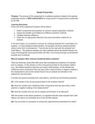
1074 Analytical Chemistry 2.0V NaOHend pointRP KHPm KHPcalibrationtemperatureend pointm KHPcalibrationbiaslinearitym KHP (tare)m KHP (gross)calibrationbiaslinearityC NaOHbiasV NaOHM KHPFigure A2.1 Cause-and-effect diagram for the standardization of NaOH by titration against KHP. The trunk, shown inblack, represents the the concentration of NaOH. The remaining arrows represent the sources of uncertainty that affectC NaOH . Light blue arrows, for example, represent the primary sources of uncertainty affecting C NaOH , and green arrowsrepresent secondary sources of uncertainty that affect the primary sources of uncertainty. See the text for additionaldetails.diagram—named for its inventor, Kaoru Ishikawa—or a fish bone diagram. To construct a cause-and-effectdiagram, we first draw an arrow pointing to the desired result; this is the diagram's trunk. We then add five mainbranch lines to the trunk, one for each of the four parameters that determine the concentration of NaOH andone for the method's repeatability. Next we add additional branches to the main branch for each of these fivefactors, continuing until we account for all potential sources of uncertainty. Figure A2.1 shows the completecause-and-effect diagram for this analysis.Before we continue, let's take a closer look at Figure A2.1 to be sure we understand each branch of thediagram. To determine the mass of KHP we make two measurements: taring the balance and weighing thegross sample. Each measurement of mass is subject to a calibration uncertainty. When we calibrate a balance,we are essentially creating a calibration curve of the balance's signal as a function of mass. Any calibration curveis subject to a systematic uncertainty in the y-intercept (bias) and an uncertainty in the slope (linearity). Wecan ignore the calibration bias because it contributes equally to both m KHP(gross) and m KHP(tare) , and becausewe determine the mass of KHP by difference.mKHP = mKHP(gross) −mKHP(tare)The volume of NaOH at the end point has three sources of uncertainty. First, an automated titrator usesa piston to deliver the NaOH to the reaction vessel, which means the volume of NaOH is subject to an uncertaintyin the piston's calibration. Second, because a solution's volume varies with temperature, there is anadditional source of uncertainty due to any fluctuation in the ambient temperature during the analysis. Finally,there is a bias in the titration's end point if the NaOH reacts with any species other than the KHP.Repeatability, R, is a measure of how consistently we can repeat the analysis. Each instrument we use—thebalance and the automatic titrator—contributes to this uncertainty. In addition, our ability to consistently

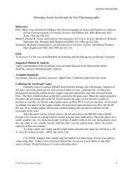
Appendices1075detect the end point also contributes to repeatability. Finally, there are no additional factors that affect theuncertainty of the KHP's purity or molar mass.Estimating the Standard Deviation for MeasurementsTo complete a propagation of uncertainty we must express each measurement’s uncertainty in the same way,usually as a standard deviation. Measuring the standard deviation for each measurement requires time andmay not be practical. Fortunately, most manufacture provides a tolerance range for glassware and instruments.A 100-mL volumetric glassware, for example, has a tolerance of ±0.1 mL at a temperature of 20 o C. We canconvert a tolerance range to a standard deviation using one of the following three approaches.Assume a Uniform Distribution. Figure A2.2a shows a uniform distribution between the limits of ±x, inwhich each result between the limits is equally likely. A uniform distribution is the choice when the manufacturerprovides a tolerance range without specifying a level of confidence and when there is no reason to believethat results near the center of the range are more likely than results at the ends of the range. For a uniformdistribution the estimated standard deviation, s, issx= 3This is the most conservative estimate of uncertainty as it gives the largest estimate for the standard deviation.Assume a Triangular Distribution. Figure A2.2b shows a triangular distribution between the limits of ±x, inwhich the most likely result is at the center of the distribution, decreasing linearly toward each limit. A triangulardistribution is the choice when the manufacturer provides a tolerance range without specifying a level ofconfidence and when there is a good reason to believe that results near the center of the range are more likelythan results at the ends of the range. For a uniform distribution the estimated standard deviation, s, issx= 6This is a less conservative estimate of uncertainty as, for any value of x, the standard deviation is smaller thanthat for a uniform distribution.Assume a Normal Distribution. Figure A2.3c shows a normal distribution that extends, as it must, beyondthe limits of ±x, and which is centered at the mid-point between –x and x. A normal distribution is the choicewhen we know the confidence interval for the range. For a normal distribution the estimated standard deviation,s, issx=zwhere z is 1.96 for a 95% confidence interval and 3.00 for a 99.7% confidence interval.(a)–x x(b)–x x(c)–x xFigure A2.2 Three possible distributions for estimating the standard deviation from a range: (a) a uniform distribution;(b) a triangular distribution; and (c) a normal distribution.

1076 Analytical Chemistry 2.0Completing the Propagation of UncertaintyNow we are ready to return to our example and determine the uncertainty for the standardization of NaOH.First we establish the uncertainty for each of the five primary sources—the mass of KHP, the volume of NaOHat the end point, the purity of the KHP, the molar mass for KHP, and the titration’s repeatability. Having establishedthese, we can combine them to arrive at the final uncertainty.Uncertainty in the Mass of KHP. After drying the KHP, we store it in a sealed container to prevent it fromreadsorbing moisture. To find the mass of KHP we first weigh the container, obtaining a value of 60.5450 g,and then weigh the container after removing a portion of KHP, obtaining a value of 60.1562 g. The mass ofKHP, therefore, is 0.3888 g, or 388.8 mg.To find the uncertainty in this mass we examine the balance’s calibration certificate, which indicates that itstolerance for linearity is ±0.15 mg. We will assume a uniform distribution because there is no reason to believethat any result within this range is more likely than any other result. Our estimate of the uncertainty for anysingle measurement of mass, u(m), is015 . mgum ( ) = = 009 . mg3Because we determine the mass of KHP by subtracting the container’s final mass from its initial mass, the uncertaintyof the mass of KHP u(m KHP ), is given by the following propagation of uncertainty.2 2um (KHP) = ( 009 . mg) + ( 0. 09 mg) = 013 . mgUncertainty in the Volume of NaOH. After placing the sample of KHP in the automatic titrator’s reaction vesseland dissolving with water, we complete the titration and find that it takes 18.64 mL of NaOH to reach theend point. To find the uncertainty in this volume we need to consider, as shown in Figure A2.1, three sourcesof uncertainty: the automatic titrator’s calibration, the ambient temperature, and any bias in determining theend point.To find the uncertainty resulting from the titrator’s calibration we examine the instrument’s certificate, whichindicates a range of ±0.03 mL for a 20-mL piston. Because we expect that an effective manufacturing processis more likely to produce a piston that operates near the center of this range than at the extremes, we will assumea triangular distribution. Our estimate of the uncertainty due to the calibration, u(V cal ) is003 . mLuV (cal) = = 0.012 mL6To determine the uncertainty due to the lack of temperature control, we draw on our prior work in the lab,which has established a temperature variation of ±3 o C with a confidence level of 95%. To find the uncertainty,we convert the temperature range to a range of volumes using water’s coefficient of expansion−4 o −1o( 21 . × 10 C )×± ( 3 C)× 1864 . mL = ± 0.012 mLand then estimate the uncertainty due to temperature, u(V temp ) as0.012 mLuV (temp) = = 0.006 mL196 .

Appendices1077Titrations using NaOH are subject to a bias due to the adsorption of CO 2 , which can react with OH – , asshown here.−−CO ( aq) + 2OH ( aq) → CO ( aq) + HO()l2 32If CO 2 is present, the volume of NaOH at the end point includes both the NaOH reacting with the KHP andthe NaOH reacting with CO 2 . Rather than trying to estimate this bias, it is easier to bathe the reaction vesselin a stream of argon, which excludes CO 2 from the titrator’s reaction vessel.Adding together the uncertainties for the piston’s calibration and the lab’s temperature fluctuation gives theuncertainty in the volume of NaOH, u(V NaOH ) as2 2uV (NaOH) = ( 0. 012 mL) + ( 0. 006 mL) = 0.013 mLUncertainty in the Purity of KHP. According to the manufacturer, the purity of KHP is 100% ± 0.05%, or1.0 ± 0.0005. Assuming a rectangular distribution, we report the uncertainty, u(P KHP ) as.uP ( ) = 0 0005=KHP0.000293Uncertainty in the Molar Mass of KHP. The molar mass of C 8 H 5 O 4 K is 204.2212 g/mol, based on the followingatomic weights: 12.0107 for carbon, 1.00794 for hydrogen, 15.9994 for oxygen, and 39.0983 for potassium.Each of these atomic weights has an quoted uncertainty that we can convert to a standard uncertaintyassuming a rectangular distribution, as shown here (the details of the calculations are left to you).element quoted uncertainty standard uncertaintycarbon ±0.0008 ±0.00046hydrogen ±0.00007 ±0.000040oxygen ±0.0003 ±0.00017potassium ±0.0001 ±0.000058Adding together the uncertainties gives the uncertainty in the molar mass, u(M KHP ), asuM ( ) = KHP8 × ( 0. 00046) 2 + 5 × ( 0. 000040) 2 + 4 × ( 0. 00017)2 + ( 0. 000058) = 0.0038 g/molUncertainty in the Titration’s Repeatability. To estimate the uncertainty due to repeatability we completefive titrations, obtaining results for the concentration of NaOH of 0.1021 M, 0.1022 M, 0.1022 M, 0.1021M, and 0.1021 M. The relative standard deviation, s r , for these titrations is5.477×10s r=0.1021−5= 0.0005If we treat the ideal repeatability as 1.0, then the uncertainty due to repeatability, u(R), is equal to the relativestandard deviation, or, in this case, 0.0005.Combining the Uncertainties. Table A2.1 summarizes the five primary sources of uncertainty. As describedearlier, we calculate the concentration of NaOH we use the following equation, which is slightly modified toinclude a term for the titration’s repeatability, which, as described above, has a value of 1.0.2

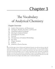
1078 Analytical Chemistry 2.0Table A2.1 Values and Uncertainties for the Standardization of NaOHsource value, x uncertainty, u(x)m KHP mass of KHP 0.3888 g 0.00013 gV NaOH volume of NaOH at end point 18.64 mL 0.013 mLP KHP purity of KHP 1.0 0.00029M KHP molar mass of KHP 204.2212 g/mol 0.0038 g/molR repeatability 1.0 0.00051000× m × PM × VKHP KHPC NaOH=KHPNaOH× RUsing the values from Table A2.1, we find that the concentration of NaOH is1000× 0. 3888×10 .C NaOH=× 10 . = 0. 1021M204. 2212×18.64Because the calculation of C NaOH includes only multiplication and division, the uncertainty in the concentration,u(C NaOH ) is given by the following propagation of uncertainty.uC (NaOH) uC (NaOH)= =C 0.1021 MNaOH( 0. 00013)2( 0.3888)222( 0. 00029)( 0. 0038)( 00 . 13)+ + +22(.) 10 ( 204. 2212)( 18. 64)22( 0. 0005)+2(.) 102Solving for u(C NaOH ) gives its value as ±0.00010 M, which is the final uncertainty for the analysis.Evaluating the Sources of UncertaintyFigure A2.3 shows the relative uncertainty in the concentration of NaOH and the relative uncertaintiesfor each of the five contributions to the total uncertainty. Of the contributions, the most important is thevolume of NaOH, and it is here to which we should focus our attention if we wish to improve the overalluncertainty for the standardization.m KHPP KHPM KHPV NaOHRC NaOHFigure A2.3 Bar graph showing the relative uncertainty inC NaOH , and the relative uncertainty in each of the mainfactors affecting the overall uncertainty.0.0000 0.0002 0.0004 0.0006 0.0008 0.0010relative uncertainty

Appendices1079Appendix 3: Single-Sided Normal DistributionThe table in this appendix gives the proportion, P, of the area under a normal distribution curve that lies tothe right of a deviation, zzX= −µσwhere X is the value for which the deviation is being defined, m is the distribution’s mean value and s is thedistribution’s standard deviation. For example, the proportion of the area under a normal distribution to theright of a deviation of 0.04 is 0.4840 (see entry in red in the table), or 48.40% of the total area (see the areashaded blue in the figure to the right). The proportion of the area to the left of the deviation is 1 – P. For adeviation of 0.04, this is 1–0.4840, or 51.60%.When the deviation is negative—that is, when X is smaller than m—the value of z is negative. In this case,the values in the table give the area to the left of z. For example, if z is –0.04, then 48.40% of the area lies tothe left of the deviation (see area shaded green in the figure shown below on the left).To use the single-sided normal distribution table, sketch the normal distribution curve for your problemand shade the area corresponding to your answer (for example, see the figure shown above on the right, which91.10%48.40%48.40%8.08%0.82%-4 -3 -2 -1 0 1 2 3Deviation (z)4230 240 250 260 270Aspirin (mg)is for Example 4.11). This divides the normal distribution curve into three regions: the area corresponding toyour answer (shown in blue), the area to the right of this, and the area to the left of this. Calculate the valuesof z for the limits of the area corresponding to your answer. Use the table to find the areas to the right and tothe left of these deviations. Subtract these values from 100% and, voilà, you have your answer.

1080 Analytical Chemistry 2.0z 0.00 0.01 0.02 0.03 0.04 0.05 0.06 0.07 0.08 0.090.0 0.5000 0.4960 0.4920 0.4880 0.4840 0.4801 0.4761 0.4721 0.4681 0.46410.1 0.4602 0.4562 0.4522 0.4483 0.4443 0.4404 0.4365 0.4325 0.4286 0.42470.2 0.4207 0.4168 0.4129 0.4090 0.4502 0.4013 0.3974 0.3396 0.3897 0.38590.3 0.3821 0.3783 0.3745 0.3707 0.3669 0.3632 0.3594 0.3557 0.3520 0.34830.4 0.3446 0.3409 0.3372 0.3336 0.3300 0.3264 0.3228 0.3192 0.3156 0.31210.5 0.3085 0.3050 0.3015 0.2981 0.2946 0.2912 0.2877 0.2843 0.2810 0.27760.6 0.2743 0.2709 0.2676 0.2643 0.2611 0.2578 0.2546 0.2514 0.2483 0.24510.7 0.2420 0.2389 0.2358 0.2327 0.2296 0.2266 0.2236 0.2206 0.2177 0.21480.8 0.2119 0.2090 0.2061 0.2033 0.2005 0.1977 0.1949 0.1922 0.1894 0.18670.9 0.1841 0.1814 0.1788 0.1762 0.1736 0.1711 0.1685 0.1660 0.1635 0.16111.0 0.1587 0.1562 0.1539 0.1515 0.1492 0.1469 0.1446 0.1423 0.1401 0.13791.1 0.1357 0.1335 0.1314 0.1292 0.1271 0.1251 0.1230 0.1210 0.1190 0.11701.2 0.1151 0.1131 0.1112 0.1093 0.1075 0.1056 0.1038 0.1020 0.1003 0.09851.3 0.0968 0.0951 0.0934 0.0918 0.0901 0.0885 0.0869 0.0853 0.0838 0.08231.4 0.0808 0.0793 0.0778 0.0764 0.0749 0.0735 0.0721 0.0708 0.0694 0.06811.5 0.0668 0.0655 0.0643 0.0630 0.0618 0.0606 0.0594 0.0582 0.0571 0.05591.6 0.0548 0.0537 0.0526 0.0516 0.0505 0.0495 0.0485 0.0475 0.0465 0.04551.7 0.0466 0.0436 0.0427 0.0418 0.0409 0.0401 0.0392 0.0384 0.0375 0.03671.8 0.0359 0.0351 0.0344 0.0336 0.0329 0.0322 0.0314 0.0307 0.0301 0.02941.9 0.0287 0.0281 0.0274 0.0268 0.0262 0.0256 0.0250 0.0244 0.0239 0.02332.0 0.0228 0.0222 0.0217 0.0212 0.0207 0.0202 0.0197 0.0192 0.0188 0.01832.1 0.0179 0.0174 0.0170 0.0166 0.0162 0.0158 0.0154 0.0150 0.0146 0.01432.2 0.0139 0.0136 0.0132 0.0129 0.0125 0.0122 0.0119 0.0116 0.0113 0.01102.3 0.0107 0.0104 0.0102 0.00964 0.00914 0.008662.4 0.00820 0.00776 0.00734 0.00695 0.006572.5 0.00621 0.00587 0.00554 0.00523 0.004942.6 0.00466 0.00440 0.00415 0.00391 0.003682.7 0.00347 0.00326 0.00307 0.00289 0.002722.8 0.00256 0.00240 0.00226 0.00212 0.001992.9 0.00187 0.00175 0.00164 0.00154 0.001443.0 0.001353.1 0.0009683.2 0.0006873.3 0.0004833.4 0.0003373.5 0.0002333.6 0.0001593.7 0.0001083.8 0.00007233.9 0.00004814.0 0.0000317

Appendix 4: Critical Values for t-TestAppendices1081Assuming you have calculated t exp , there are two approaches to interpreting a t-test. In the first approach youchoose a value of a for rejecting the null hypothesis and read the value of t(a,n) from the table shown below.If t exp >t(a,n), you reject the null hypothesis and accept the alternative hypothesis. In the second approach,you find the row in the table below corresponding to your degrees of freedom and move across the row to find(or estimate) the a corresponding to t exp = t(a,n); this establishes largest value of a for which you can retainthe null hypothesis. Finding, for example, that a is 0.10 means that you would retain the null hypothesis atthe 90% confidence level, but reject it at the 89% confidence level. The examples in this textbook use the firstapproach.Values of t for……a confidence interval of: 90% 95% 98% 99%…an a value of: 0.10 0.05 0.02 0.01Degrees of Freedom1 6.314 12.706 31.821 63.6572 2.920 4.303 6.965 9.9253 2.353 3.182 4.541 5.8414 2.132 2.776 3.747 4.6045 2.015 2.571 3.365 4.0326 1.943 2.447 3.143 3.7077 1.895 2.365 2.998 3.4998 1.860 2.306 2.896 3.2559 1.833 2.262 2.821 3.25010 1.812 2.228 2.764 3.16912 1.782 2.179 2.681 3.05514 1.761 2.145 2.624 2.97716 1.746 2.120 2.583 2.92118 1.734 2.101 2.552 2.87820 1.725 2.086 2.528 2.84530 1.697 2.042 2.457 2.75050 1.676 2.009 2.311 2.678∞ 1.645 1.960 2.326 2.576The values in this table are for a two-tailed t-test. For a one-tail t-test, divide the a values by 2. For example, thelast column has an a value of 0.005 and a confidence interval of 99.5% when conducting a one-tailed t-test.

1082 Analytical Chemistry 2.0Appendix 5: Critical Values for the F-TestThe following tables provide values for F(0.05, n num , n denom ) for one-tailed and for two-tailed F-tests. To usethese tables, decide whether the situation calls for a one-tailed or a two-tailed analysis and calculate F expFss2= Aexp 2Bwhere s A 2 is greater than s B 2 . Compare F exp to F(0.05, n num , n denom ) and reject the null hypothesis if F exp >F(0.05, n num , n denom ). You may replace s with s if you know the population’s standard deviation.F(0.05, n num , n denom ) for a One-Tailed F-Testonum&0 odenom1 2 3 4 5 6 7 8 9 10 15 20 ∞1 161.4 199.5 215.7 224.6 230.2 234.0 236.8 238.9 240.5 241.9 245.9 248.0 254.32 18.51 19.00 19.16 19.25 19.30 19.33 19.35 19.37 19.38 19.40 19.43 19.45 19.503 10.13 9.552 9.277 9.117 9.013 8.941 8.887 8.845 8.812 8.786 8.703 8.660 8.5264 7.709 6.994 6.591 6.388 6.256 6.163 6.094 6.041 5.999 5.964 5.858 5.803 5.6285 6.608 5.786 5.409 5.192 5.050 4.950 4.876 4.818 4.722 4.753 4.619 4.558 4.3656 5.591 5.143 4.757 4.534 4.387 4.284 4.207 4.147 4.099 4.060 3.938 3.874 3.6697 5.591 4.737 4.347 4.120 3.972 3.866 3.787 3.726 3.677 3.637 3.511 3.445 3.2308 5.318 4.459 4.066 3.838 3.687 3.581 3.500 3.438 3.388 3.347 3.218 3.150 2.9289 5.117 4.256 3.863 3.633 3.482 3.374 3.293 3.230 3.179 3.137 3.006 2.936 2.70710 4.965 4.103 3.708 3.478 3.326 3.217 3.135 3.072 3.020 2.978 2.845 2.774 2.53811 4.844 3.982 3.587 3.257 3.204 3.095 3.012 2.948 2.896 2.854 2.719 2.646 2.40412 4.747 3.885 3.490 3.259 3.106 2.996 2.913 2.849 2.796 2.753 2.617 2.544 2.29613 4.667 3.806 3.411 3.179 3.025 2.915 2.832 2.767 2.714 2.671 2.533 2.459 2.20614 4.600 3.739 3.344 3.112 2.958 2.848 2.764 2.699 2.646 2.602 2.463 2.388 2.13115 4.534 3.682 3.287 3.056 2.901 2.790 2.707 2.641 2.588 2.544 2.403 2.328 2.06616 4.494 3.634 3.239 3.007 2.852 2.741 2.657 2.591 2.538 2.494 2.352 2.276 2.01017 4.451 3.592 3.197 2.965 2.810 2.699 2.614 2.548 2.494 2.450 2.308 2.230 1.96018 4.414 3.555 3.160 2.928 2.773 2.661 2.577 2.510 2.456 2.412 2.269 2.191 1.91719 4.381 3.552 3.127 2.895 2.740 2.628 2.544 2.477 2.423 2.378 2.234 2.155 1.87820 4,351 3.493 3.098 2.866 2.711 2.599 2.514 2.447 2.393 2.348 2.203 2.124 1.843∞ 3.842 2.996 2.605 2.372 2.214 2.099 2.010 1.938 1.880 1.831 1.666 1.570 1.000

Appendices1083F(0.05, n num , n denom ) for a Two-Tailed F-Testonum&0 odenom1 2 3 4 5 6 7 8 9 10 15 20 ∞1 647.8 799.5 864.2 899.6 921.8 937.1 948.2 956.7 963.3 968.6 984.9 993.1 10182 38.51 39.00 39.17 39.25 39.30 39.33 39.36 39.37 39.39 39.40 39.43 39.45 39.503 17.44 16.04 15.44 15.10 14.88 14.73 14.62 14.54 14.47 14.42 14.25 14.17 13.904 12.22 10.65 9.979 9.605 9.364 9.197 9.074 8.980 8.905 8.444 8.657 8.560 8.2575 10.01 8.434 7.764 7.388 7.146 6.978 6.853 6.757 6.681 6.619 6.428 6.329 6.0156 8.813 7.260 6.599 6.227 5.988 5.820 5.695 5.600 5.523 5.461 5.269 5.168 4.8947 8.073 6.542 5.890 5.523 5.285 5.119 4.995 4.899 4.823 4.761 4.568 4.467 4.1428 7.571 6.059 5.416 5.053 4.817 4.652 4.529 4.433 4.357 4.259 4.101 3.999 3.6709 7.209 5.715 5.078 4.718 4.484 4.320 4.197 4.102 4.026 3.964 3.769 3.667 3.33310 6.937 5.456 4.826 4.468 4.236 4.072 3.950 3.855 3.779 3.717 3.522 3.419 3.08011 6.724 5.256 4.630 4.275 4.044 3.881 3.759 3.644 3.588 3.526 3.330 3.226 2.88312 6.544 5.096 4.474 4.121 3.891 3.728 3.607 3.512 3.436 3.374 3.177 3.073 2.72513 6.414 4.965 4.347 3.996 3.767 3.604 3.483 3.388 3.312 3.250 3.053 2.948 2.59614 6.298 4.857 4.242 3.892 3.663 3.501 3.380 3.285 3.209 3.147 2.949 2.844 2.48715 6.200 4.765 4.153 3.804 3.576 3.415 3.293 3.199 3.123 3.060 2.862 2.756 2.39516 6.115 4.687 4.077 3.729 3.502 3.341 3.219 3.125 3.049 2.986 2.788 2.681 2.31617 6.042 4.619 4.011 3.665 3.438 3.277 3.156 3.061 2.985 2.922 2.723 2.616 2.24718 5.978 4.560 3.954 3.608 3.382 3.221 3.100 3.005 2.929 2.866 2.667 2.559 2.18719 5.922 4.508 3.903 3.559 3.333 3.172 3.051 2.956 2.880 2.817 2.617 2.509 2.13320 5.871 4.461 3.859 3.515 3.289 3.128 3.007 2.913 2.837 2.774 2.573 2.464 2.085∞ 5.024 3.689 3.116 2.786 2.567 2.408 2.288 2.192 2.114 2.048 1.833 1.708 1.000

1084 Analytical Chemistry 2.0Appendix 6: Critical Values for Dixon’s Q-TestThe following table provides critical values for Q(a, n), where a is the probability of incorrectly rejecting thesuspected outlier and n is the number of samples in the data set. There are several versions of Dixon’s Q-Test,each of which calculates a value for Q ij where i is the number of suspected outliers on one end of the data setand j is the number of suspected outliers on the opposite end of the data set. The values given here are for Q 10 ,whereQ = Q = outliersvalue ' − nearest valueexp 10largest value−smallest valueThe suspected outlier is rejected if Q exp is greater than Q(a, n). For additional information consult Rorabacher,D. B. “Statistical Treatment for Rejection of Deviant Values: Critical Values of Dixon’s ‘Q’ Parameter and RelatedSubrange Ratios at the 95% confidence Level,” Anal. Chem. 1991, 63, 139–146.Critical Values for the Q-Test of a Single Outlier (Q 10 )a &0 n 0.1 0.05 0.04 0.02 0.013 0.941 0.970 0.976 0.988 0.9944 0.765 0.829 0.846 0.889 0.9265 0.642 0.710 0.729 0.780 0.8216 0.560 0.625 0.644 0.698 0.7407 0.507 0.568 0.586 0.637 0.6808 0.468 0.526 0.543 0.590 0.6349 0.437 0.493 0.510 0.555 0.59810 0.412 0.466 0.483 0.527 0.568

AppendicesAppendix 7: Critical Values for Grubb’s Test1085The following table provides critical values for G(a, n), where a is the probability of incorrectly rejectingthe suspected outlier and n is the number of samples in the data set. There are several versions of Grubb’s Test,each of which calculates a value for G ij where i is the number of suspected outliers on one end of the data setand j is the number of suspected outliers on the opposite end of the data set. The values given here are for G 10 ,whereG = X XoutG = −exp 10sThe suspected outlier is rejected if G exp is greater than G(a, n).G(a, n) for Grubb’s Test of a Single Outliera0 &n0.05 0.013 1.155 1.1554 1.481 1.4965 1.715 1.7646 1.887 1.9737 2.202 2.1398 2.126 2.2749 2.215 2.38710 2.290 2.48211 2.355 2.56412 2.412 2.63613 2.462 2.69914 2.507 2.75515 2.549 2.755

1086 Analytical Chemistry 2.0Appendix 8: Recommended Primary StandardsAll compounds should be of the highest available purity. Metals should be cleaned with dilute acid to removeany surface impurities and rinsed with distilled water. Unless otherwise indicated, compounds should be driedto a constant weight at 110 o C. Most of these compounds are soluble in dilute acid (1:1 HCl or 1:1 HNO 3 ),with gentle heating if necessary; some of the compounds are water soluble.Element Compound FW (g/mol) Commentsaluminum Al metal 26.982antimony Sb metal 121.760KSbOC 4 H 4 O 6 324.92 prepared by drying KSbC 4 H 4 O 6 •1/2H 2 O at110 o C and storing in a desiccatorarsenic As metal 74.922As 2 O 3 197.84 toxicbarium BaCO 3 197.84 dry at 200 o C for 4 hbismuth Bi metal 208.98boron H 3 BO 3 61.83 do not drybromine KBr 119.01cadmium Cd metal 112.411CdO 128.40calcium CaCO 3 100.09cerium Ce metal 140.116(NH 4 ) 2 Ce(NO 3 ) 4 548.23cesium Cs 2 CO 3 325.82Cs 2 SO 4 361.87chlorine NaCl 58.44chromium Cr metal 51.996K 2 Cr 2 O 7 294.19cobalt Co metal 58.933copper Cu metal 63.546CuO 79.54fluorine NaF 41.99 do not store solutions in glass containersiodine KI 166.00KIO 3 214.00iron Fe metal 55.845lead Pb metal 207.2lithium Li 2 CO 3 73.89magnesium Mg metal 24.305manganese Mn metal 54.938

Appendices1087Element Compound FW (g/mol) Commentsmercury Hg metal 200.59molybdenum Mo metal 95.94nickel Ni metal 58.693phosphorous KH 2 PO 4 136.09P 2 O 5 141.94potassium KCl 74.56K 2 CO 3 138.21K 2 Cr 2 O 7 294.19KHC 8 H 4 O 2 204.23silicon Si metal 28.085SiO 2 60.08silver Ag metal 107.868AgNO 3 169.87sodium NaCl 58.44Na 2 CO 3 106.00Na 2 C2O 4 134.00strontium SrCO 3 147.63sulfur elemental S 32.066K 2 SO 4 174.27Na 2 SO 4 142.04tin Sn metal 118.710titanium Ti metal 47.867tungsten W metal 183.84uranium U metal 238.029U 3 O 8 842.09vanadium V metal 50.942zinc Zn metal 81.37Sources: (a) Smith, B. W.; Parsons, M. L. J. Chem. Educ. 1973, 50, 679–681; (b) Moody, J. R.; Greenburg, P.R.; Pratt, K. W.; Rains, T. C. Anal. Chem. 1988, 60, 1203A–1218A.

1088 Analytical Chemistry 2.0Appendix 9: Correcting Massfor the Buoyancy of AirCalibrating a balance does not eliminate all sources of determinate error in the signal. Because of the buoyancyof air, an object always weighs less in air than it does in a vacuum. If there is a difference between theobject’s density and the density of the weights used to calibrate the balance, then we can make a correction forbuoyancy. 1 An object’s true weight in vacuo, W v , is related to its weight in air, W a , by the equationWv1 1= Wa# > 1 + f - p#0 . 0012H D DA9.1owhere D o is the object’s density, D w is the density of the calibration weight, and 0.0012 is the density of airunder normal laboratory conditions (all densities are in units of g/cm 3 ). The greater the difference between D oand D w the more serious the error in the object’s measured weight.The buoyancy correction for a solid is small, and frequently ignored. It may be significant, however, forlow density liquids and gases. This is particularly important when calibrating glassware. For example, we cancalibrate a volumetric pipet by carefully filling the pipet with water to its calibration mark, dispensing the waterinto a tared beaker, and determining the water’s mass. After correcting for the buoyancy of air, we use thewater’s density to calculate the volume dispensed by the pipet.ExampleA 10-mL volumetric pipet was calibrated following the procedure just outlined, using a balance calibratedwith brass weights having a density of 8.40 g/cm 3 . At 25 o C the pipet dispensed 9.9736 g of water. What isthe actual volume dispensed by the pipet and what is the determinate error in this volume if we ignore thebuoyancy correction? At 25 o C the density of water is 0.997 05 g/cm 3 .So l u t i o nUsing equation A9.1 the water’s true weight is1 1W v= 9 . 9736 g # > 1 + e - o # 0 . 0012H = 9 . 9842 g0 . 99705 8 . 40wand the actual volume of water dispensed by the pipet is9.9842 g0.99705 g/cm33= 10. 014 cm = 10.014 mLIf we ignore the buoyancy correction, then we report the pipet’s volume as9.9736 g0.99705 g/cmintroducing a negative determinate error of -0.11%.33= 10. 003 cm = 10.003 mL1 Battino, R.; Williamson, A. G. J. Chem. Educ. 1984, 61, 51–52.

Appendices1089Pr o b l e m sThe following problems will help you in considering the effect of buoyancy on the measurement of mass.1. In calibrating a 10-mL pipet a measured volume of water was transferred to a tared flask and weighed,yielding a mass of 9.9814 grams. (a) Calculate, with and without correcting for buoyancy, the volume ofwater delivered by the pipet. Assume that the density of water is 0.99707 g/cm3 and that the density ofthe weights is 8.40 g/cm3. (b) What are the absolute and relative errors introduced by failing to accountfor the effect of buoyancy? Is this a significant source of determinate error for the calibration of a pipet?Explain.2. Repeat the questions in problem 1 for the case where a mass of 0.2500 g is measured for a solid that has adensity of 2.50 g/cm3.3. Is the failure to correct for buoyancy a constant or proportional source of determinate error?4. What is the minimum density of a substance necessary to keep the buoyancy correction to less than 0.01%when using brass calibration weights with a density of 8.40 g/cm3?

1090 Analytical Chemistry 2.0Appendix 10: Solubility ProductsThe following table provides pK sp and K sp values for selected compounds, organized by the anion. All valuesare from Martell, A. E.; Smith, R. M. Critical Stability Constants, Vol. 4. Plenum Press: New York, 1976. Unlessotherwise stated, values are for 25 o C and zero ionic strength.Bromide (Br – ) pK sp K spCuBr 8.3 5.×10 –9AgBr 12.30 5.0×10 –13Hg 2 Br 2 22.25 5.6×10 –13HgBr 2 (m = 0.5 M) 18.9 1.3×10 –19PbBr 2 (m = 4.0 M) 5.68 2.1×10 –6Carbonate (CO 2– 3 ) pK sp K spMgCO 3 7.46 3.5×10 –8CaCO 3 (calcite) 8.35 4.5×10 –9CaCO 3 (aragonite) 8.22 6.0×10 –9SrCO 3 9.03 9.3×10 –10BaCO 3 8.30 5.0×10 –9MnCO 3 9.30 5.0×10 –10FeCO 3 10.68 2.1×10 –11CoCO 3 9.98 1.0×10 –10NiCO 3 6.87 1.3×10 –7Ag 2 CO 3 11.09 8.1×10 –12Hg 2 CO 3 16.05 8.9×10 –17ZnCO 3 10.00 1.0×10 –10CdCO 3 13.74 1.8×10 –14PbCO 3 13.13 7.4×10 –14Chloride (Cl – ) pK sp K spCuCl 6.73 1.9×10 –7AgCl 9.74 1.8×10 –10Hg 2 Cl 2 17.91 1.2×10 –18PbCl 2 4.78 2.0×10 –19

Appendices1091Chromate (CrO 2– 4 ) pK sp K spBaCrO 4 9.67 2.1×10 –10CuCrO 4 5.44 3.6×10 –6Ag 2 CrO 4 11.92 1.2×10 –12Hg 2 CrO 4 8.70 2.0×10 –9Cyanide (CN – ) pK sp K spAgCN 15.66 2.2×10 –16Zn(CN) 2 (m = 3.0 M) 15.5 3.×10 –16Hg 2 (CN) 2 39.3 5.×10 –40Ferrocyanide [Fe(CN) 4– 6 ] pK sp K spZn 2 [Fe(CN) 6 ] 15.68 2.1×10 –16Cd 2 [Fe(CN) 6 ] 17.38 4.2×10 –18Pb 2 [Fe(CN) 6 ] 18.02 9.5×10 –19Fluoride (F – ) pK sp K spMgF 2 8.18 6.6×10 –9CaF 2 10.41 3.9×10 –11SrF 2 8.54 2.9×10 –9BaF 2 5.76 1.7×10 –6PbF 2 7.44 3.6×10 –8Hydroxide (OH – ) pK sp K spMg(OH) 2 11.15 7.1×10 –12Ca(OH) 2 5.19 6.5×10 –6Ba(OH) 2 •8H 2 O 3.6 3.×10 –4La(OH) 3 20.7 2.×10 –21Mn(OH) 2 12.8 1.6×10 –13Fe(OH) 2 15.1 8.×10 –16Co(OH) 2 14.9 1.3×10 –15Ni(OH) 2 15.2 6.×10 –16Cu(OH) 2 19.32 4.8×10 –20Fe(OH) 3 38.8 1.6×10 –39

Appendices1093Pb 3 (PO 4 ) 2 (T = 38 o C) 43.55 3.0×10 –44Sulfate (SO 2– 4 ) pK sp K spCaSO 4 4.62 2.4×10 –5SrSO 4 6.50 3.2×10 –7BaSO 4 9.96 1.1×10 –10Ag 2 SO 4 4.83 1.5×10 –5Hg 2 SO 4 6.13 7.4×10 –7PbSO 4 7.79 1.6×10 –8Sulfide (S 2– ) pK sp K spMnS (green) 13.5 3.×10 –14FeS 18.1 8.×10 –19CoS (b) 25.6 3.×10 –26NiS (g) 26.6 3.×10 –27CuS 36.1 8.×10 –37Cu 2 S 48.5 3.×10 –49Ag 2 S 50.1 8.×10 –51ZnS (a) 24.7 2.×10 –25CdS 27.0 1.×10 –27Hg 2 S (red) 53.3 5.×10 –54PbS 27.5 3.×10 –28Thiocyanate (SCN – ) pK sp K spCuSCN (m = 5.0 M) 13.40 4.0×10 –14AgSCN 11.97 1.1×10 –12Hg 2 (SCN) 2 19.52 3.0×10 –20Hg(SCN) 2 (m = 1.0 M) 19.56 2.8×10 –20

1094 Analytical Chemistry 2.0Appendix 11: Acid Dissociation ConstantsThe following table provides pK a and K a values for selected weak acids. All values are from Martell, A. E.;Smith, R. M. Critical Stability Constants, Vols. 1–4. Plenum Press: New York, 1976. Unless otherwise stated,values are for 25 o C and zero ionic strength. Those values in brackets are considered less reliable.Weak acids are arranged alphabetically by the names of the neutral compounds from which they are derived. Insome cases—such as acetic acid—the compound is the weak acid. In other cases—such as for the ammoniumion—the neutral compound is the conjugate base. Chemical formulas or structural formulas are shown forthe fully protonated weak acid. Successive acid dissociation constants are provided for polyprotic weak acids;where there is ambiguity, the specific acidic proton is identified.To find the K b value for a conjugate weak base, recall thatK a × K b = K wfor a conjugate weak acid, HA, and its conjugate weak base, A – .Compound Conjugate Acid pK a K aacetic acid CH 3 COOH 4.757 1.75×10 –5adipic acidHOOOOH4.425.423.8×10 –53.8×10 –6alanineO+ H 3 N CH CCH 3OH2.348 (COOH)9.867 (NH 3 )4.49×10 –31.36×10 –10aminobenzene NH 3+4.601 2.51×10 –54-aminobenzene sulfonic acid NH 3+O 3 S 3.232 5.86×10 –42-aminobenozic acidCOOHNH 3+2.08 (COOH)4.96 (NH 3 )8.3×10 –31.1×10 –52-aminophenol (T = 20 o C)ammonia NH 4+OHNH 3+4.78 (NH 3 )9.97 (OH)1.7×10 –51.05×10 –109.244 5.70×10 –10

Appendices1095Compound Conjugate Acid pK a K aO+ H 3 N CH COHarginineCH 2CH 2CH 2NH1.823 (COOH)8.991 (NH 3 )[12.48] (NH 2 )1.50×10 –21.02×10 –9[3.3×10 –13 ]CNH 2+NH 3+arsenic acid H 3 AsO 4 6.962.2411.50asparagine (m = 0.1 M)+ H 3 N CH CCH 2OC ONH 2OH2.14 (COOH)8.72 (NH 3 )5.8×10 –31.1×10 –73.2×10 –127.2×10 –31.9×10 –9Oasparatic acid+ H 3 N CH CCH 2C OOHOH1.990 (a-COOH)3.900 (b-COOH)10.002 (NH 3 )1.02×10 –21.26×10 –49.95×10 –11benzoic acid COOH 4.202 6.28×10 –5benzylamine CH 2 NH 3+9.35 4.5×10 –10boric acid (pK a2 , pK a3 :T = 20 o C) H 3 BO 3 [12.74]9.236[13.80]carbonic acid H 2 CO 36.35210.329catecholOHOH9.4012.85.81×10 –10[1.82×10 –13 ][1.58×10 –14 ]4.45×10 –74.69×10 –114.0×10 –101.6×10 –13chloroacetic acid ClCH 2 COOH 2.865 1.36×10 –3chromic acid (pK a1 :T = 20 o C) H 2 CrO 4-0.26.511.63.1×10 –7

1096 Analytical Chemistry 2.0Compound Conjugate Acid pK a K aCOOH3.128 (COOH) 7.45×10 –4citric acidHOOCCOOH 4.761 (COOH) 1.73×10 –5OH6.396 (COOH) 4.02×10 –7cupferrron (m = 0.1 M)cysteineN+ H 3 N CH CCH 2SHNOOHOOH4.16 6.9×10 –5[1.71] (COOH)8.36 (SH)10.77 (NH 3 )[1.9×10 –2 ]4.4×10 –91.7×10 –11dichloracetic acid Cl 2 CHCOOH 1.30 5.0×10 –2diethylamine (CH 3 CH 2 ) 2 NH 2+dimethylamine (CH 3 ) 2 NH 2+dimethylglyoximeHONNOHethylamine CH 3 CH 2 NH 3+ethylenediamineethylenediaminetetraacetic acid(EDTA) (m = 0.1 M)HOOCHOOC10.933 1.17×10 –1110.774 1.68×10 –1110.6612.0+ H 3 NCH 2 CH 2 NH 3+ 6.8489.928NH ++ HNCOOHCOOH2.2×10 –111.×10 –1210.636 2.31×10 –110.0 (COOH)1.5 (COOH)2.0 (COOH)2.66 (COOH)6.16 (NH)10.24 (NH)1.42×10 –71.18×10 –101.03.2×10 –21.0×10 –22.2×10 –36.9×10 –75.8×10 –11formic acid HCOOH 3.745 1.80×10 –4fumaric acidHOOCOCOOH3.0534.4948.85×10 –43.21×10 –5glutamic acid+ H 3 N CH CCH 2CH 2C OOH2.33 (a-COOH)4.42 (l-COOH)9.95 (NH 3 )5.9×10 –33.8×10 –51.12×10 –10OH

Appendices1097Compound Conjugate Acid pK a K aO+ H 3 N CH COHglutamine (m = 0.1 M)CH 2CH 22.17 (COOH)9.01 (NH 3 )6.8×10 –39.8×10 –10C ONH 2glycine + H 3 NCH 2 COOH + H 3 N CH CHOOH2.350 (COOH)9.778 (NH 3 )4.47×10 –31.67×10 –10glycolic acid HOOCH 2 COOH 3.831 (COOH) 1.48×10 –4Ohistidine (m = 0.1 M)+ H 3 N CH CCH 2+ HNOH1.7 (COOH)6.02 (NH)9.08 (NH 3 )2.×10 –29.5×10 –78.3×10 –10NHhydrogen cyanide HCN 9.21 6.2×10 –10hydrogen fluoride HF 3.17 6.8×10 –4hydrogen peroxide H 2 O 2 11.65 2.2×10 –12hydrogen sulfideH 2 S7.0213.99.5×10 –81.3×10 –14hydrogen thiocyanate HSCN 0.9 1.3×10 –18-hydroxyquinolineOHNH +hydroxylamine HONH 3+4.91 (NH)9.81 (OH)1.2×10 –51.6×10 –105.96 1.1×10 –6hypobromous acid HOBr 8.63 2.3×10 –9hypochlorous acid HOCl 7.53 3.0×10 –8hypoiodous acid HOI 10.64 2.3×10 –11iodic acid HIO 3 0.77 1.7×10 –1Oisoleucine+ H 3 N CH C OHCH CH 3CH 22.319 (COOH)9.754 (NH 3 )4.80×10 –31.76×10 –10CH 3

Compound Conjugate Acid pK a K aOleucine+ H 3 N CH CCH 2OHCH CH 32.329 (COOH)9.747 (NH 3 )4.69×10 –31.79×10 –10CH 3O+ H 3 N CH COHlysine (m = 0.1 M)CH 2CH 2CH 22.04 (COOH)9.08 (a-NH 3 )10.69 (e-NH 3 )9.1×10 –38.3×10 –102.0×10 –11CH 2NH 3+maleic acidmalic acidmalonic acidHOOC COOH 1.9106.332HOOCOHCOOHHOOCCH 2 COOHO3.459 (COOH)5.097 (COOH)2.8475.6969.1×10 –39.1×10 –39.1×10 –39.1×10 –39.1×10 –39.1×10 –3+ H 3 N CH COHmethionine (m = 0.1 M)CH 2CH 22.20 (COOH)9.05 (NH 3 )9.1×10 –39.1×10 –3SCH 3methylamine CH 3 NH 3+10.64 9.1×10 –32-methylanalineNH 3+4.447 9.1×10 –34-methylanaline NH 3+5.084 9.1×10 –32-methylphenolOH10.28 9.1×10 –34-methylphenol OH 10.26 9.1×10 –3

Appendices1099Compound Conjugate Acid pK a K aCOOHnitrilotriacetic acid (T = 20 o C)(pK a1 : m = 0.1 m) NH +HOOC COOH2-nitrobenzoic acidCOOHCOOH1.1 (COOH)1.650 (COOH)2.940 (COOH)10.334 (NH 3 )9.1×10 –39.1×10 –39.1×10 –39.1×10 –3NO 22.179 9.1×10 –33-nitrobenzoic acid4-nitrobenzoic acidNO 23.449 9.1×10 –3O 2 N COOH 3.442 3.61×10 –42-nitrophenolOHNO 27.21 6.2×10 –8OH3-nitrophenol4-nitrophenolNO 28.39 4.1×10 –9O 2 N OH 7.15 7.1×10 –8nitrous acid HNO 2 3.15 7.1×10 –4oxalic acid H 2 C 2 O 41.2524.2665.60×10 –25.42×10 –51,10-phenanthroline4.86 1.38×10 –5NH +Nphenol OH 9.98 1.05×10 –10

1100 Analytical Chemistry 2.0Compound Conjugate Acid pK a K aphenylalanine+ H 3 N CH CCH 2OOH2.20 (COOH)9.31 (NH 3 )6.3×10 –34.9×10 –10phosphoric acid H 3 PO 4 7.1992.14812.35phthalic acidCOOHCOOH2.9505.4087.11×10 –36.32×10 –84.5×10 –131.12×10 –33.91×10 –6piperdine NH 2+11.123 7.53×10 –12prolineNH 2+COOH1.952 (COOH)10.640 (NH)1.12×10 –22.29×10 –11propanoic acid CH 3 CH 2 COOH 4.874 1.34×10 –5propylamine CH 3 CH 2 CH 2 NH 3+10.566 2.72×10 –11pryidine NH + 5.229 5.90×10 –6resorcinolOHOH9.3011.065.0×10 –108.7×10 –12salicylic acidCOOHOH2.97 (COOH)13.74 (OH)1.1×10 –31.8×10 –14serinesuccinic acid+ H 3 N CH CHOOCCH 2OHOOHCOOH2.187 (COOH)9.209 (NH 3 )4.2075.636sulfuric acid H 2 SO 4strong1.996.50×10 –36.18×10 –106.21×10 –52.31×10 –6—1.0×10 –2

Appendices1101Compound Conjugate Acid pK a K a1.91sulfurous acid H 2 SO1.2×10 –237.186.6×10 –8d-tartaric acidHOOCOHOHCOOH3.036 (COOH)4.366 (COOH)9.20×10 –44.31×10 –5Othreonine+ H 3 N CH C OHCH OH2.088 (COOH)9.100 (NH 3 )8.17×10 –37.94×10 –10CH 3thiosulfuric acid H 2 S 2 O 30.61.63.×10 –13.×10 –2trichloroacetic acid (m = 0.1 M) Cl 3 CCOOH 0.66 2.2×10 –1triethanolamine (HOCH 2 CH 2 ) 3 NH + 7.762 1.73×10 –8triethylamine (CH 3 CH 2 ) 3 NH + 10.715 1.93×10 –11trimethylamine (CH 3 ) 3 NH + 9.800 1.58×10 –10tris(hydroxymethyl)amino methane(TRIS or THAM)tryptophan (m = 0.1 M)(HOCH 2 ) 3 CNH 3++ H 3 N CH CHNCH 2OOH8.075 8.41×10 –92.35 (COOH)9.33 (NH 3 )4.5×10 –34.7×10 –10O+ H 3 N CH COHtryosine (pK a1 : m = 0.1 M)CH 22.17 (COOH)9.19 (NH 3 )10.47 (OH)6.8×10 –36.5×10 –103.4×10 –11OHOvaline+ H 3 N CH C OHCH CH 32.286 (COOH)9.718 (NH 3 )5.18×10 –31.91×10 –10CH 3

1102 Analytical Chemistry 2.0Appendix 12: Formation ConstantsThe following table provides K i and b i values for selected metal–ligand complexes, arranged by the ligand.All values are from Martell, A. E.; Smith, R. M. Critical Stability Constants, Vols. 1–4. Plenum Press: NewYork, 1976. Unless otherwise stated, values are for 25 o C and zero ionic strength. Those values in brackets areconsidered less reliable.AcetateCH 3 COO – log K 1 log K 2 log K 3 log K 4 log K 5 log K 6Mg 2+ 1.27Ca 2+ 1.18Ba 2+ 1.07Mn 2+ 1.40Fe 2+ 1.40Co 2+ 1.46Ni 2+ 1.43Cu 2+ 2.22 1.41Ag 2+ 0.73 –0.09Zn 2+ 1.57Cd 2+ 1.93 1.22 –0.89Pb 2+ 2.68 1.40AmmoniaNH 3 log K 1 log K 2 log K 3 log K 4 log K 5 log K 6Ag + 3.31 3.91Co 2+ (T = 20 o C) 1.99 1.51 0.93 0.64 0.06 –0.73Ni 2+ 2.72 2.17 1.66 1.12 0.67 –0.03Cu 2+ 4.04 3.43 2.80 1.48Zn 2+ 2.21 2.29 2.36 2.03Cd 2+ 2.55 2.01 1.34 0.84ChlorideCl – log K 1 log K 2 log K 3 log K 4 log K 5 log K 6Cu 2+ 0.40Fe 3+ 1.48 0.65Ag + (m = 5.0 M) 3.70 1.92 0.78 –0.3Zn 2+ 0.43 0.18 –0.11 –0.3Cd 2+ 1.98 1.62 –0.2 –0.7Pb 2+ 1.59 0.21 –0.1 –0.3

Appendices1103CyanideCN – log K 1 log K 2 log K 3 log K 4 log K 5 log K 6Fe 2+ 35.4 (b 6 )Fe 3+ 43.6 (b 6 )Ag + 20.48 b 2 0.92Zn 2+ 11.07 b 2 4.98 3.57Cd 2+ 6.01 5.11 4.53 2.27Hg 2+ 17.00 15.75 3.56 2.66Ni 2+ 30.22 (b 4 )EthylenediamineH 2 NNH 2 log K 1 log K 2 log K 3 log K 4 log K 5 log K 6Ni 2+ 7.38 6.18 4.11Cu 2+ 10.48 9.07Ag + (T = 20 o C, m = 0.1 M) 4.700 3.00Zn 2+ 5.66 4.98 3.25Cd 2+ 5.41 4.50 2.78EDTAOOCCOONNOOCCOOlog K 1 log K 2 log K 3 log K 4 log K 5 log K 6Mg 2+ (T = 20 o C, m = 0.1 M) 8.79Ca 2+ (T = 20 o C, m = 0.1 M) 10.69Ba 2+ (T = 20 o C, m = 0.1 M) 7.86Bi 3+ (T = 20 o C, m = 0.1 M) 27.8Co 2+ + (T = 20 o C, m = 0.1 M) 16.31Ni 2+ (T = 20 o C, m = 0.1 M) 18.62Cu 2+ (T = 20 o C, m = 0.1 M) 18.80Cr 3+ (T = 20 o C, m = 0.1 M) [23.4]Fe 3+ (T = 20 o C, m = 0.1 M) 25.1Ag + (T = 20 o C, m = 0.1 M) 7.32Zn 2+ (T = 20 o C, m = 0.1 M) 16.50Cd 2+ (T = 20 o C, m = 0.1 M) 16.46Hg 2+ (T = 20 o C, m = 0.1 M) 21.7Pb 2+ (T = 20 o C, m = 0.1 M) 18.04

1104 Analytical Chemistry 2.0Al 3+ (T = 20 o C, m = 0.1 M) 16.3FluorideF – log K 1 log K 2 log K 3 log K 4 log K 5 log K 6Al 3+ (m = 0.5 M) 6.11 5.01 3.88 3.0 1.4 0.4HydroxideOH – log K 1 log K 2 log K 3 log K 4 log K 5 log K 6Al 3+ 9.01 [9.69] [8.3] 6.0Co 2+ 4.3 4.1 1.3 0.5Fe 2+ 4.5 [2.9] 2.6 –0.4Fe 3+ 11.81 10.5 12.1Ni 2+ 4.1 3.9 3.Pb 2+ 6.3 4.6 3.0Zn 2+ 5.0 [6.1] 2.5 [1.2]IodideI – log K 1 log K 2 log K 3 log K 4 log K 5 log K 6Ag + (T = 18 o C) 6.58 [5.12] [1.4]Cd 2+ 2.28 1.64 1.08 1.0Pb 2+ 1.92 1.28 0.7 0.6NitriloacetateCOONOOC COO log K 1 log K 2 log K 3 log K 4 log K 5 log K 6Mg 2+ (T = 20 o C, m = 0.1 M) 5.41Ca 2+ (T = 20 o C, m = 0.1 M) 6.41Ba 2+ (T = 20 o C, m = 0.1 M) 4.82Mn 2+ (T = 20 o C, m = 0.1 M) 7.44Fe 2+ (T = 20 o C, m = 0.1 M) 8.33Co 2+ (T = 20 o C, m = 0.1 M) 10.38Ni 2+ (T = 20 o C, m = 0.1 M) 11.53Cu 2+ (T = 20 o C, m = 0.1 M) 12.96Fe 3+ (T = 20 o C, m = 0.1 M) 15.9Zn 2+ (T = 20 o C, m = 0.1 M) 10.67

Appendices1105Cd 2+ (T = 20 o C, m = 0.1 M) 9.83Pb 2+ (T = 20 o C, m = 0.1 M) 11.39Oxalate2–C 2 O 4 log K 1 log K 2 log K 3 log K 4 log K 5 log K 6Ca 2+ (m = 1 M) 1.66 1.03Fe 2+ (m = 1 M) 3.05 2.10Co 2+ 4.72 2.28Ni 2+ 5.16Cu 2+ 6.23 4.04Fe 3+ (m = 0.5 M) 7.53 6.11 4.85Zn 2+ 4.87 2.781,10-PhenanthrolineN N log K 1 log K 2 log K 3 log K 4 log K 5 log K 6Fe 2+ 20.7 (b 3 )Mn 2+ (m = 0.1 M) 4.0 3.3 3.0Co 2+ (m = 0.1 M) 7.08 6.64 6.08Ni 2+ 8.6 8.1 7.6Fe 3+ 13.8 (b 3 )Ag + (m = 0.1 M) 5.02 7.04Zn 2+ 6.2 [5.9] [5.2]Thiosulfate2–S 2 O 3 log K 1 log K 2 log K 3 log K 4 log K 5 log K 6Ag + (T = 20 o C) 8.82 4.85 0.53ThiocyanateSCN – log K 1 log K 2 log K 3 log K 4 log K 5 log K 6Mn 2+ 1.23Fe 2+ 1.31Co 2+ 1.72Ni 2+ 1.76Cu 2+ 2.33Fe 3+ 3.02

1106 Analytical Chemistry 2.0Ag + 4.8 3.43 1.27 0.2Zn 2+ 1.33 0.58 0.09 –0.4Cd 2+ 1.89 0.89 0.02 –0.5Hg 2+ 17.26 (b 2 ) 2.71 1.83

AppendicesAppendix 13: Standard Reduction PotentialsThe following table provides E o and E o´ values for selected reduction reactions. Values are from the followingsources: Bard, A. J.; Parsons, B.; Jordon, J., eds. Standard Potentials in Aqueous Solutions, Dekker: New York,1985; Milazzo, G.; Caroli, S.; Sharma, V. K. Tables of Standard Electrode Potentials, Wiley: London, 1978; Swift,E. H.; Butler, E. A. Quantitative Measurements and Chemical Equilibria, Freeman: New York, 1972.Solids, gases, and liquids are identified; all other species are aqueous. Reduction reactions in acidic solution arewritten using H + in place of H 3 O + . You may rewrite a reaction by replacing H + with H 3 O + and adding to theopposite side of the reaction one molecule of H 2 O per H + ; thusbecomesH 3 AsO 4 + 2H + + 2e – HAsO 2 + 2H 2 OH 3 AsO 4 + 2H 3 O + + 2e – HAsO 2 + 4H 2 OConditions for formal potentials (E o´) are listed next to the potential.Aluminum E° (V) E°’(V)Al+ 3e Al() s–1.6763+ −Al(OH) − 4+ 3e− Al() s + 4OH−–2.3103AlF − + 3e− Al() s + 6F−–2.0761107Antimony E° (V) E°’(V)Sb + 3H + + 3e− SbH3( g ) –0.510Sb2O5() s + 6H + 4e 2SbO + 3H2O()l0.605+ + −SbO + 2H + 3e Sb() s + HO() l0.2122Arsenic E° (V) E°’(V)As + 3H + + 3e− AsH3( g ) –0.225+HAsO + 2H + 2e− HAsO + 2H O() l0.5603 4 2 2+HAsO 2+ 3H + 3e − As() s + 2H 2O() l0.240Barium E° (V) E°’(V)Ba+ 2e Ba() s–2.922+ −BaO() s + 2H + + 2e− Ba() s + HO()l2.3652

1108 Analytical Chemistry 2.0Beryllium E° (V) E°’(V)Be+ 2e Be() s–1.992+ −Bismuth E° (V) E°’(V)Bi+ 3e Bi() s0.3173+ −BiCl − 4+ 3e− Bi() s + 4Cl−0.199Boron E° (V) E°’(V)+B(OH) 3+ 3H + 3e B() s + 3HO2() l–0.890B(OH) 4+ 3e B()s + 4OH–1.811Bromine E° (V) E°’(V)Br2e 2Br1.0872 + − −HOBr + H + + 2e− Br − + H O() l1.3412HOBr + H + + e− 1 Br −2 + H O() l1.6042BrO + H O()l + 2e Br + 2OH− − − −20.76 in 1 M NaOHBrO − + 6H + + 5e− Br () l + 3HO1.531 2 2− + − −BrO 3+ 6H + 6e Br + 3HO21.4782Cadmium E° (V) E°’(V)Cd+ 2e Cd() s–0.40302+ −2Cd(CN) − + 2e− Cd() s + 4CN−–0.94342Cd(NH ) + + 2e− Cd() s + 4NH–0.6223 43Calcium E° (V) E°’(V)Ca+ 2e Ca() s–2.842+ −

Appendices1109Carbon E° (V) E°’(V)CO 2( g) + 2H + 2eCO( g) + H 2O()l–0.106CO 2( g ) + 2H + 2eHCO 2H–0.202CO ( g ) + 2H + + 2e− H CO–0.4812 2 2 4HCHO + 2H + + 2e − CHOH30.2323Cerium E° (V) E°’(V)Ce+ 3e Ce() s–2.3363+ −Ce+ e Ce1.724+ − 3+1.70 in 1 M HClO 41.44 in 1 M H 2 SO 41.61 in 1 M HNO 31.28 in 1 M HClChlorine E° (V) E°’(V)Cl2( g ) + 2e 2Cl1.396ClO − + H O() l + e − 1 Cl ( g)+ OH−2 22 0.421 in 1 M NaOH2ClO + H O()l + 2e Cl + 2OH− − − −20.890 in 1 M NaOH+HClO 2+ 2H + 2e − HOCl+H 2O1.64ClO − + 2H + + e− ClO ( g ) + H O1.1753 2− + −ClO + 3H + 2e HClO + HO1.1813 2− + − −ClO + 2H + 2e ClO + H O1.2014 3222Chromium E° (V) E°’(V)CrCr+ e Cr–0.4243+ − 2++ 2e Cr() s–0.902+ −Cr O − + 14H + + 6e− 2Cr + + 7HO() l1.362 72 322CrO − + 4H O() l + 3e − 2CrOH ( )− + 4OH−–0.13 in 1 M NaOH424

1110 Analytical Chemistry 2.0Cobalt E° (V) E°’(V)CoCo+ 2e Co() s–0.2772+ −+ e Co1.923+ − 2+Co(NH3+ − 2+) + e Co(NH )0.13 63 6−−Co(OH) () s + e Co(OH)() s + OH0.173 2−−Co(OH) 2() s + 2e Co()s + 2OH–0.746Copper E° (V) E°’(V)CuCuCu+ e Cu() s0.520+ −+ e Cu0.1592+ − ++ 2e Cu() s0.34192+ −2+ − −Cu + I +e CuI() s0.862+ − −Cu + Cl +e CuCl() s0.559Fluorine E° (V) E°’(V)F2 ( g ) + 2H + 2e2HF3.053F2 ( g ) ++ 2e 2F2.87Gallium E° (V) E°’(V)Ga+ 3e Ga()s3+ −Gold E° (V) E°’(V)AuAuAu+ e Au() s1.83+ −+ 2e Au1.363+ − ++ 3e Au() s1.523+ −AuCl − 4+ 3e− Au() s + 4Cl−1.002

Appendices1111Hydrogen E° (V) E°’(V)+ −2H+ 2e H2( g ) 0.00000−−HO2+ e 1 2H2 ( g + OH–0.828Iodine E° (V) E°’(V)I2()s + 2e 2I0.5355I3+ 2e 3I0.536HIO+ H + + 2e− I − + H O() l0.9852− + −IO + 6H + 5e I () s + 3HO() l1.19531 2 22IO − 3+ 3HO 2() l + 6e − I − + 6OH−0.257Iron E° (V) E°’(V)Fe+ 2e Fe() s–0.442+ −FeFe+ 3e Fe() s–0.0373+ −+ e Fe0.7713+ − 2+Fe(CN)4+ e Fe(CN)0.3563− − −660.70 in 1 M HCl0.767 in 1 M HClO 40.746 in 1 M HNO 30.68 in 1 M H 2 SO 40.44 in 0.3 M H 3 PO 4Fe(phen)2+ e Fe(phen)1.1473+ − +66Lanthanum E° (V) E°’(V)La+ 3e La() s–2.383+ −Lead E° (V) E°’(V)Pb+ 2e Pb() s–0.1262+ −PbO () s + 4OH − + 2e− Pb + + 2H O()l1.4622PbO () s + 4SO − + 4H + + 2e− PbSO () s + 2H O()l 1.6902 42−2−PbSO () s + 2e Pb()s + SO–0.3564 4242

1112 Analytical Chemistry 2.0Lithium E° (V) E°’(V)Li+ e Li() s–3.040+ −Magnesium E° (V) E°’(V)Mg+ 2e Mg() s–2.3562+ −−−Mg(OH)2() s + 2e Mg()s + 2OH–2.687Manganese E° (V) E°’(V)MnMn+ 2e Mn() s–1.172+ −+ e Mn1.53+ − 2+MnO () s + 4H + + 2e− Mn + + 2HO()l1.2322− + −MnO + 4H + 3e MnO () s + 2H O() l1.704 2MnO − + 8H + + 5e− Mn + + 4HO() l1.5142MnO − + 2H O() l + 3e − MnO () s + 4OH−0.604 22222Mercury E° (V) E°’(V)Hg+ 2e Hg() l0.85352+ −2+ − 2+2Hg+ 2e Hg0.911Hg2+ 2e 2Hg() l0.79602+ −2−−Hg2Cl2() s + 2e 2Hg()l + 2Cl0.2682HgO() s + 2H + + 2e− Hg() l + HO()l0.926−−Hg2Br2() s + 2e 2Hg()l + 2Br1.392−−Hg2I2() s + 2e 2Hg()l + 2I–0.04052

Appendices1113Molybdenum E° (V) E°’(V)Mo+ 3e Mo() s–0.23+ −MoO 2() s + 4H + + 4e− Mo() s + 2HO2() l–0.1522MoO − + 4H O() l + 6e − Mo()s + 8OH−–0.91342Nickel E° (V) E°’(V)Ni+ 2e Ni() s–0.2572+ −−−Ni( OH) 2+ 2e Ni()s + 2OH–0.722Ni( NH ) + + 2e− Ni()s + 6NH–0.493 63Nitrogen E° (V) E°’(V)N ( g ) + 5H + + 4e− NH+–0.232 2 5NO( g) + 2H + + 2e− N ( g) + HO()l1.772 22NO( g) + 2H + 2eN2O( g) + H 2O()l1.59+HNO 2+ H + e − NO( g) + HO 2() l0.9962HNO + 4H + + 4e − NO( g) + 3HO() l1.2972 2− + −NO3 + 3H + 2e HNO2+H2O() l0.9422Oxygen E° (V) E°’(V)O 2( g ) + 2H + 2eHO 2 20.695O 2( g) + 4H + 4e2HO2() l1.229HO 2 2+ 2H + 2e 2H 2O() l1.763O2( g) + 2H2O()l + 4e 4OH0.401O ( g) + 2H + + 2e− O ( g) + H O()l2.073 22

1114 Analytical Chemistry 2.0Phosphorous E° (V) E°’(V)P(, s white) + 3H + + 3e− PH3( g)+ −HPO + 2H + 2e HPO + H O()l3 3 3 2 2HPO + 2H + + 2e− HPO + H O()l3 4 3 3 2Platinum E° (V) E°’(V)Pt+ 2e Pt()s2+ −2PtCl + 2e Pt()s + 4Cl− − −4Potassium E° (V) E°’(V)K+ e K()s+ −Ruthenium E° (V) E°’(V)Ru+ e Ru0.2493+ − 2+RuO 2() s + 4H + + 4e− Ru() s + 2HO2() l0.683+ − 2+Ru( NH ) + e Ru()s + Ru( NH )0.103 63− − 4−Ru( CN) + e Ru()s + Ru( CN)0.86663 6Selenium E° (V) E°’(V)Se()s + e22 Se–0.67 in 1 M NaOHSe() s + 2H + + 2e− H2Se( g)–0.115+HSeO 2 3+ 4H + 4e Se() s + 3H 2O() l0.74SeO − + 4H + + e− HSeO + HO() l1.151432 32Silicon E° (V) E°’(V)2SiF − + 4e− Si() s + 6F−–1.376SiO 2() s + 4H + + 4e− Si() s + 2HO2() l–0.909SiO () s + 8H + + 8e− SiH ( g) + 2H O()l–0.5162 42

Appendices1115Silver E° (V) E°’(V)Ag+ e Ag() s0.7996+ −−−AgBr() s + e Ag()s + Br0.071−2−Ag CO() s + 2e 2Ag()s + CO0.472 2 4 2 4−−AgCl() s + e Ag()s + Cl0.2223−−AgI() s + e Ag()s + I–0.152−2−Ag S() s + 2e 2Ag()s + S–0.712+ −Ag( NH ) + e Ag()s + 2NH–0.3733 2 3Sodium E° (V) E°’(V)Na+ e Na() s–2.713+ −Strontium E° (V) E°’(V)Sr+ 2e Sr() s–2.892+ −Sulfur E° (V) E°’(V)S()s + e22 S–0.407S()s + 2H + + 2e− HS20.1442− + −SO + 4H + 2e 2H SO0.5692 6SO2 32+ 2e 2SO1.962− − −2 84SO2+ 2e 2SO0.0802− − −4 62 3222SO − + 2HO()l + 2e − SO − + 4OH−–1.13322 4222SO − + 3HO()l + 4e − SO − + 6OH−–0.576 in 1 M NaOH322 32− + − 2−2SO + 4H + 2e S O + 2H O() l–0.2542 62SO − 2+ HO()l + 2e − SO − + 2OH−–0.936423SO − 2+ 4H + ++ 2e− H SO − + HO() l0.172422 322

1116 Analytical Chemistry 2.0Thallium E° (V) E°’(V)TlTl+ 2e Tl3+ − ++ 3e Tl() s0.7423+ −1.25 in 1 M HClO 40.77 in 1 M HClTin E° (V) E°’(V)SnSn+ 2e Sn() s–0.19 in 1 M HCl2+ −+ 2e Sn0.154 0.139 in 1 M HCl4+ − 2+Titanium E° (V) E°’(V)TiTi+ 2e Ti() s–0.1632+ −+ e Ti–0.373+ − 2+Tungsten E° (V) E°’(V)WO 2() s + 4H + 4eW() s + 2HO2() l–0.119WO 3() s + 6H + 6eW() s + 3HO2() l–0.090Uranium E° (V) E°’(V)UU+ 3e U() s–1.663+ −+ e U–0.524+ − 3+UO + + 4H + + e− U + + 2HO() l0.27UO242+ e UO0.162+ − +22UO + + 4H + + 2e− U + + 2HO() l0.32722 42Vanadium E° (V) E°’(V)VV+ 2e V() s–1.132+ −+ e V–0.2553+ − 2+2VO + 3+ 2H + + e− V + + HO() l0.3372VO + + 2H + + e− VO + + H O() l1.00022 22

Appendices1117Zinc E° (V) E°’(V)Zn+ 2e Zn() s–0.76182+ −2Zn(OH) − + 2e− Zn() s + 4OH−–1.28542Zn(NH ) + + 2e− Zn() s + 4NH–1.043 42−−Zn(CN) + 2e Zn() s + 4CN–1.3443

1118 Analytical Chemistry 2.0Appendix 14: Random Number TableThe following table provides a list of random numbers in which the digits 0 through 9 appear with approximatelyequal frequency. Numbers are arranged in groups of five to make the table easier to view. This arrangementis arbitrary, and you can treat the table as a sequence of random individual digits (1, 2, 1, 3, 7, 4…goingdown the first column of digits on the left side of the table), as a sequence of three digit numbers (111, 212,104, 367, 739… using the first three columns of digits on the left side of the table), or in any other similarmanner.Let’s use the table to pick 10 random numbers between 1 and 50. To do so, we choose a random starting point,perhaps by dropping a pencil onto the table. For this exercise, we will assume that the starting point is the fifthrow of the third column, or 12032. Because the numbers must be between 1 and 50, we will use the last twodigits, ignoring all two-digit numbers less than 01 or greater than 50, and rejecting any duplicates. Proceedingdown the third column, and moving to the top of the fourth column when necessary, gives the following 10random numbers: 32, 01, 05, 16, 15, 38, 24, 10, 26, 14.These random numbers (1000 total digits) are a small subset of values from the publication Million RandomDigits (Rand Corporation, 2001) and used with permission. Information about the publication, and a link toa text file containing the million random digits is available at http://www.rand.org/pubs/monograph_reports/MR1418/.11164 36318 75061 37674 26320 75100 10431 20418 19228 9179221215 91791 76831 58678 87054 31687 93205 43685 19732 0846810438 44482 66558 37649 08882 90870 12462 41810 01806 0297736792 26236 33266 66583 60881 97395 20461 36742 02852 5056473944 04773 12032 51414 82384 38370 00249 80709 72605 6749749563 12872 14063 93104 78483 72717 68714 18048 25005 0415164208 48237 41701 73117 33242 42314 83049 21933 92813 0476351486 72875 38605 29341 80749 80151 33835 52602 79147 0886899756 26360 64516 17971 48478 09610 04638 17141 09227 1060671325 55217 13015 72907 00431 45117 33827 92873 02953 8547465285 97198 12138 53010 95601 15838 16805 61004 43516 1702017264 57327 38224 29301 31381 38109 34976 65692 98566 2955095639 99754 31199 92558 68368 04985 51092 37780 40261 1447961555 76404 86210 11808 12841 45147 97438 60022 12645 6200078137 98768 04689 87130 79225 08153 84967 64539 79493 7491762490 99215 84987 28759 19177 14733 24550 28067 68894 3849024216 63444 21283 07044 92729 37284 13211 37485 10415 3645716975 95428 33226 55903 31605 43817 22250 03918 46999 9850159138 39542 71168 57609 91510 77904 74244 50940 31553 6256229478 59652 50414 31966 87912 87514 12944 49862 96566 48825

Appendix 15: PolarographicHalf-Wave PotentialsAppendicesThe following table provides E 1/2 values for selected reduction reactions. Values are from Dean, J. A. AnalyticalChemistry Handbook, McGraw-Hill: New York, 1995.AlCdCrCoCoCuFeFePbMnNiZnElement E 1/2 (volts vs. SCE) Matrix+ 3e Al() s–0.5 0.2 M acetate (pH 4.5–4.7)3+ −+ 2e Cd() s–0.602+ −+ 3e Cr()s3+ −+ 3e Co()s3+ −–0.35 (+3 → +2)–1.70 (+2 → 0)–0.5 (+3 → +2)–1.3 (+2 → 0)+ 2e Co() s–1.03 1 M KSCN2+ −+ 2e Cu()s2+ −+ 3e Fe()s3+ −0.04–0.22–0.17 (+3 → +2)–1.52 (+2 → 0)0.1 M KCl0.05 M H 2 SO 41 M HNO 31 M NH 4 Cl plus 1 M NH 31 M NH + 4 /NH 3 buffer (ph 8–9)1 M NH 4 Cl plus 1 M NH 30.1 M KSCN0.1 M NH 4 ClO 41 M Na 2 SO 40.5 M potassium citrate (pH 7.5)0.5 M sodium tartrate (pH 5.8)+ e Fe–0.27 0.2 M Na 2 C 2 O 4 (pH < 7.9)3+ − 2++ 2e Pb()s2+ −–0.405–0.4351 M HNO 31 M KCl+ 2e Mn() s–1.65 1 M NH 4 Cl plus 1 M NH 32+ −+ 2e Ni()s2+ −+ 2e Zn()s2+ −–0.70–1.09–0.995–1.331 M KSCN1 M NH 4 Cl plus 1 M NH 30.1 M KCl1 M NH 4 Cl plus 1 M NH 31119

1120 Analytical Chemistry 2.0Appendix 16: Countercurrent SeparationsIn 1949, Lyman Craig introduced an improved method for separating analytes with similar distribution ratios. 1The technique, which is known as a countercurrent liquid–liquid extraction, is outlined in Figure A16.1 anddiscussed in detail below. In contrast to a sequential liquid–liquid extraction, in which we repeatedly extractthe sample containing the analyte, a countercurrent extraction uses a serial extraction of both the sample andthe extracting phases. Although countercurrent separations are no longer common—chromatographic separationsare far more efficient in terms of resolution, time, and ease of use—the theory behind a countercurrentextraction remains useful as an introduction to the theory of chromatographic separations.To track the progress of a countercurrent liquid-liquid extraction we need to adopt a labeling convention.As shown in Figure A16.1, in each step of a countercurrent extraction we first complete the extraction andthen transfer the upper phase to a new tube containing a portion of the fresh lower phase. Steps are labeledsequentially beginning with zero. Extractions take place in a series of tubes that also are labeled sequentially,starting with zero. The upper and lower phases in each tube are identified by a letter and number, with theletters U and L representing, respectively, the upper phase and the lower phase, and the number indicating thestep in the countercurrent extraction in which the phase was first introduced. For example, U 0 is the upperphase introduced at step 0 (during the first extraction), and L 2 is the lower phase introduced at step 2 (duringthe third extraction). Finally, the partitioning of analyte in any extraction tube results in a fraction p remainingin the upper phase, and a fraction q remaining in the lower phase. Values of q are calculated using equationA16.1, which is identical to equation 7.26 in Chapter 7.( q )aq1( molesaq) V1aq= =( molesaq) DV + V0orgaqA16.1The fraction p, of course is equal to 1 – q. Typically V aq and V org are equal in a countercurrent extraction, althoughthis is not a requirement.Let’s assume that the analyte we wish to isolate is present in an aqueous phase of 1 M HCl, and that theorganic phase is benzene. Because benzene has the smaller density, it is the upper phase, and 1 M HCl is thelower phase. To begin the countercurrent extraction we place the aqueous sample containing the analyte in tube0 along with an equal volume of benzene. As shown in Figure A16.1a, before the extraction all the analyte ispresent in phase L 0 . When the extraction is complete, as shown in Figure A16.1b, a fraction p of the analyte ispresent in phase U 0 , and a fraction q is in phase L 0 . This completes step 0 of the countercurrent extraction. If westop here, there is no difference between a simple liquid–liquid extraction and a countercurrent extraction.After completing step 0, we remove phase U 0 and add a fresh portion of benzene, U 1 , to tube 0 (see FigureA16.1c). This, too, is identical to a simple liquid-liquid extraction. Here is where the power of the countercurrentextraction begins—instead of setting aside the phase U 0 , we place it in tube 1 along with a portion ofanalyte-free aqueous 1 M HCl as phase L 1 (see Figure A16.1c). Tube 0 now contains a fraction q of the analyte,and tube 1 contains a fraction p of the analyte. Completing the extraction in tube 0 results in a fraction p ofits contents remaining in the upper phase, and a fraction q remaining in the lower phase. Thus, phases U 1and L 0 now contain, respectively, fractions pq and q 2 of the original amount of analyte. Following the samelogic, it is easy to show that the phases U 0 and L 1 in tube 1 contain, respectively, fractions p 2 and pq of analyte.This completes step 1 of the extraction (see Figure A16.1d). As shown in the remainder of Figure A16.1, thecountercurrent extraction continues with this cycle of phase transfers and extractions.1 Craig, L. C. J. Biol. Chem. 1944, 155, 519–534.

Appendices1121(a)U 00L 01extract(b)U 0pL 0qtransfernewphase(c)U 10U 0pL 0qnewphaseL 10extractextract(d)U 1pqU 0p2L 0q2transferL 1pqtransfernewphase(e)U 20U 1pqU 0p2L 0q2L 1pqnewphaseL 20newphaseextract(f)(g)U 2pq2L 0q3U 30L 0q3transferextractU 12p2qL 12pq2U 2pq2L 12pq2transferextractU 0p3L 2p2qU 12p2qL 2p2qtransfernewphaseU 0p3Tube 0 Tube 1 Tube 2 Tube 3L 30Figure A16.1 Scheme for a countercurrentextraction: (a) The sample containing theanalyte begins in L 0 and is extracted with afresh portion of the upper, or mobile phase;(b) The extraction takes place, transferring afraction p of analyte to the upper phase andleaving a fraction q of analyte in the lower,or stationary phase; (c) When the extractionis complete, the upper phase is transferred tothe next tube, which contains a fresh portionof the sample’s solvent, and a fresh portionof the upper phase is added to tube 0. In (d)through (g), the process continues, with theaddition of two more tubes.

1122 Analytical Chemistry 2.0Table A16.1 Fraction of Analyte Remaining in Tube r After Extraction Step n for aCountercurrent Extractionn↓ r→ 0 1 2 30 1 — — —1 q p — —2 q 2 2pq p 2 —3 q 3 3pq 2 3p 2 q p 3In a countercurrent liquid–liquid extraction, the lower phase in each tube remains in place, and the upperphase moves from tube 0 to successively higher numbered tubes. We recognize this difference in the movementof the two phases by referring to the lower phase as a stationary phase and the upper phase as a mobile phase.With each transfer some of the analyte in tube r moves to tube r + 1, while a portion of the analyte in tube r – 1moves to tube r. Analyte introduced at tube 0 moves with the mobile phase, but at a rate that is slower thanthe mobile phase because, at each step, a portion of the analyte transfers into the stationary phase. An analytethat preferentially extracts into the stationary phase spends proportionally less time in the mobile phase andmoves at a slower rate. As the number of steps increases, analytes with different values of q eventually separateinto completely different sets of extraction tubes.We can judge the effectiveness of a countercurrent extraction using a histogram showing the fraction ofanalyte present in each tube. To determine the total amount of analyte in an extraction tube we add togetherthe fraction of analyte present in the tube’s upper and lower phases following each transfer. For example, at thebeginning of step 3 (see Figure A16.1g) the upper and lower phases of tube 1 contain fractions pq 2 and 2pq 2of the analyte, respectively; thus, the total fraction of analyte in the tube is 3pq 2 . Table A16.1 summarizes thisfor the steps outlined in Figure A16.1. A typical histogram, calculated assuming distribution ratios of 5.0 foranalyte A and 0.5 for analyte B, is shown in Figure A16.2. Although four steps is not enough to separate the(a)1.0(b) 1.0Figure A16.2 Progress of a countercurrent extractionfor the separation of analytes A and B showing thefraction of anlayte in each tube after (a) step 0, (b) step1, (c) step 2, and (d) step 3. The distribution ratio, D,is 5.0 for analyte A and 0.5 for analyte B. The volumesof the two phases are identical.fraction of analyte(c)fraction of analyte0.80.60.40.20.01.00.80.60.40.20.0analyte Aanalyte Bfraction of analyte fraction of analyte0.80.60.40.20.00 1 2 3 0 1 2 3tube numbertube number(d) 1.00.80.60.40.20.00 1 2 3 0 1 2 3tube numbertube number

Appendices1123analytes in this instance, it is clear that if we extend the countercurrent extraction to additional tubes, we willeventually separate the analytes.Figure A16.1 and Table A16.1 show how an analyte’s distribution changes during the first four steps of acountercurrent extraction. Now we consider how we can generalize these results to calculate the amount ofanalyte in any tube, at any step during the extraction. You may recognize the pattern of entries in Table A16.1as following the binomial distributionn!−f (, r n)= pq( n − r)! r !r n rA16.2where f(r, n) is the fraction of analyte present in tube r at step n of the countercurrent extraction, with theupper phase containing a fraction p f(r, n) of analyte and the lower phase containing a fraction qf(r, n) ofthe analyte.Example A16.1The countercurrent extraction shown in Figure A16.2 is carried out through step 30. Calculate the fraction ofanalytes A and B in tubes 5, 10, 15, 20, 25, and 30.So l u t i o nTo calculate the fraction, q, for each analyte in the lower phase we use equation A6.1. Because the volumes ofthe lower and upper phases are equal, we getqA1=D + = 11 5+ 1= 0. 167 qAB1=D + = 11 4+ 1=B0.200Because we know that p + q = 1, we also know that p A is 0.833 and that p B is 0.333. For analyte A, the fractionin tubes 5, 10, 15, 20, 25, and 30 after the 30 th step aref (, 530 30!)( )! ! ( . )( 50 833 030 5 5 . 167 ) 30−5== 21 . × 10−−15≈ 0f ( 10 !, 30 30)( )! ! ( . ) 100 83330 10 10 ( 0 . 167 ) 30−10== 1−. −94× 10 ≈0f ( 15 !, 30 30)( )! ! ( . ) 150 83330 15 15 ( 0 . 167 ) 30−15== 2−. −52× 10 ≈0f ( 20 !, 30 30)( )! ! ( . ) 200 83330 20 20 ( 0 . 167 ) 30−20== 0−. 013f ( 25 !, 30 30)( )! ! ( . ) 250 83330 25 25 ( 0 . 167 ) 30−25== 0−. 192f ( 30 !, 30 30)( )! ! ( . ) 300 83330 30 30 ( 0 . 167 ) 30−30== 0−. 004

1124 Analytical Chemistry 2.00.200.180.16analyte Aanalyte BFigure A16.3 Progress of a countercurrent extractionfor the separation of analyte A and Bshowing the fraction of analyte in each tube after30 steips. The distribution ratio, D, is 5.0 foranalyte A and 0.5 for analyte B. The volumes ofthe two phases are identical. See Example A16.1for further details.fraction of analyte0.140.120.100.080.060.040.020.000 5 10 15 20 25 30tube numberThe fraction of analyte B in tubes 5, 10, 15, 20, 25, and 30 is calculated in the same way, yielding respectivevalues of 0.023, 0.153, 0.025, 0, 0, and 0. Figure A16.3, which provides the complete histogram for the distributionof analytes A and B, shows that 30 steps is sufficient to separate the two analytes.Constructing a histogram using equation A16.2 is tedious, particularly when the number of steps is large.Because the fraction of analyte in most tubes is approximately zero, we can simplify the histogram’s constructionby solving equation A16.2 only for those tubes containing an amount of analyte exceeding a thresholdvalue. For a binomial distribution, we can use the mean and standard deviation to determine which tubescontain a significant fraction of analyte. The properties of a binomial distribution were covered in Chapter 4,with the mean, µ, and the standard deviation, s, given asµ = npσ= np( 1− p)= npqFurthermore, if both np and nq are greater than 5, the binomial distribution is closely approximated by thenormal distribution and we can use the properties of a normal distribution to determine the location of theanalyte and its recovery. 2Example A16.2Two analytes, A and B, with distribution ratios of 9 and 4, respectively, are separated using a countercurrentextraction in which the volumes of the upper and lower phases are equal. After 100 steps determine the 99%confidence interval for the location of each analyte.2 Mark, H.; Workman, J. Spectroscopy 1990, 5(3), 55–56.

Appendices1125So l u t i o nThe fraction, q, of each analyte remaining in the lower phase is calculated using equation A16.1. Because thevolumes of the lower and upper phases are equal, we find thatqqAB1=D + = 11 9+ 1=A1=D + = 11 4+ 1=BBecause we know that p + q = 1, we also know that p A is 0.90 and p B is 0.80. After 100 steps, the mean andthe standard deviation for the distribution of analytes A and B are010 .020 .µ = np = ( 100)( 090 . ) = 90 and σ = np q = ( 100)( 090 . )( 010 . )= 3A A A A Aµ = np = ( 100)( 080 . ) = 80 and σ = np q = ( 100)( 080 . )( 020 . )= 4B B B B BGiven that np A , np B , nq A , and nq B are all greater than 5, we can assume that the distribution of analytes followsa normal distribution and that the confidence interval for the tubes containing each analyte isr = µ ± zswhere r is the tube’s number and the value of z is determined by the desired significance level. For a 99%confidence interval the value of z is 2.58 (Appendix 4); thus,r A = 90 ± (2.58)(3) = 90 ± 8r B = 80 ± (2.58)(4) = 80 ± 10Because the two confidence intervals overlap, a complete separation of the two analytes is not possible using a100 step countercurrent extraction. The complete distribution of the analytes is shown in Figure A16.4.0.150.12analyte Aanalyte Bfraction of analyte0.090.060.030.0065 70 75 80 85 90 95 100tube numberFigure A16.4 Progress of the countercurrent extraction in ExampleA16.2 after 100 steps. Although analyte A moves more quicklythan analyte B, the similarity of their distribution ratios, and thusthe similarity in their values of q, means the separation of analytesA and B is not yet complete.

1126 Analytical Chemistry 2.0Example A16.3For the countercurrent extraction in Example A16.2, calculate the recovery and separation factor for analyteA if the contents of tubes 85–99 are pooled together.So l u t i o nFrom Example A16.2 we know that after 100 steps of the countercurrent extraction, analyte A is normallydistributed about tube 90 with a standard deviation of 3. To determine the fraction of analyte A in tubes 85–99,we use the single-sided normal distribution in Appendix 3 to determine the fraction of analyte in tubes 0–84,and in tube 100. The fraction of analyte A in tube 100 is determined by calculating the deviation zrz = − µ 99= − 90= 3σ 3and using the table in Appendix 3 to determine the corresponding fraction. For z = 3 this corresponds to0.135% of analyte A. To determine the fraction of analyte A in tubes 0–84 we again calculate the deviationrz = − µ 85= − 90=−167.σ 3From Appendix 3 we find that 4.75% of analyte A is present in tubes 0–84. Analyte A’s recovery, therefore,is100% – 4.75% – 0.135% ≈ 95%To calculate the separation factor we determine the recovery of analyte B in tubes 85–99 using the same generalapproach as for analyte A, finding that approximately 89.4% of analyte B remains in tubes 0–84 and thatessentially no analyte B is in tube 100. The recover for B, therefore, isand the separation factor is100% – 89.4% – 0% ≈ 10.6%SB,ARA10.6= = = 0.112R 95B

AppendicesAppendix 17: Review of Chemical KineticsA reaction’s equilibrium position defines the extent to which the reaction can occur. For example, we expecta reaction with a large equilibrium constant, such as the dissociation of HCl in water+ −HCl( aq) + H O() l H O ( aq) + ( aq)2 3Clto proceed nearly to completion. A large equilibrium constant, however, does not guarantee that a reactionwill reach its equilibrium position. Many reactions with large equilibrium constants, such as the reduction ofMnO 4 – by H 2 O4MnO – −( aq) + 2H O() l 4MnO () s + 3O ( g) + 4OH( aq)4 22 2do not occur to an appreciable extent. The study of the rate at which a chemical reaction approaches its equilibriumposition is called kinetics.A17.1 Chemical Reaction RatesA study of a reaction’s kinetics begins with the measurement of its reaction rate. Consider, for example, thegeneral reaction shown below, involving the aqueous solutes A, B, C, and D, with stoichiometries of a, b, c,and d.aA+ bB cC+dDA17.1The rate, or velocity, at which this reaction approaches its equilibrium position is determined by following thechange in concentration of one reactant or one product as a function of time. For example, if we monitor theconcentration of reactant A, we express the rate asdR =− [A] A17.2dtwhere R is the measured rate expressed as a change in concentration of A as a function of time. Because a reactant’sconcentration decreases with time, we include a negative sign so that the rate has a positive value.We also can determine the rate by following the change in concentration of a product as a function of time,which we express asd[C]R′ =−A17.3dtRates determined by monitoring different species do not necessarily have the same value. The rate R in equationA17.2 and the rate R´ in equation A17.3 have the same value only if the stoichiometric coefficients of A andC in reaction A17.1 are identical. In general, the relationship between the rates R and R´ isA17.2 The Rate LawaR = × R′cA rate law describes how a reaction’s rate is affected by the concentration of each species in the reaction mixture.The rate law for reaction A17.1 takes the general form of1127

1128 Analytical Chemistry 2.0α β γ δR = k[ A] [ B] [ C] [ D][ E]ε A17.4where k is the rate constant, and a, b, g, d, and e are the reaction orders of the reaction for each species presentin the reaction.There are several important points about the rate law in equation A17.4. First, a reaction’s rate may dependon the concentrations of both reactants and products, as well as the concentration of a species that does notappear in the reaction’s overall stoichiometry. Species E in equation A17.4, for example, may be a catalyst thatdoes not appear in the reaction’s overall stoichiometry, but which increases the reaction’s rate. Second, the reactionorder for a given species is not necessarily the same as its stoichiometry in the chemical reaction. Reactionorders may be positive, negative, or zero, and may take integer or non-integer values. Finally, the reaction’soverall reaction order is the sum of the individual reaction orders for each species. Thus, the overall reactionorder for equation A17.4 is a + b + g + d + e.A17.3 Kinetic Analysis of Selected ReactionsIn this section we review the application of kinetics to several simple chemical reactions, focusing on how wecan use the integrated form of the rate law to determine reaction orders. In addition, we consider how we candetermine the rate law for a more complex system.Fi r s t-Or d e r Re a c t i o n sThe simplest case we can treat is a first-order reaction in which the reaction’s rate depends on the concentrationof only one species. The best example of a first-order reaction is an irreversible thermal decomposition ofa single reactant, which we represent aswith a rate law ofA→ ProductsA17.5d[A]R =− = k[A] A17.6dtThe simplest way to demonstrate that a reaction is first-order in A, is to double the concentration of A andnote the effect on the reaction’s rate. If the observed rate doubles, then the reaction must be first-order in A.Alternatively, we can derive a relationship between the concentration of A and time by rearranging equationA17.6 and integrating.[ A] t∫d[A]kdt[ A] =−td[A]=−kdt[ A]∫A17.7[ A] 0 0Evaluating the integrals in equation A17.7 and rearrangingln [ A]t[ A]0=−ktA17.8ln[ A] =− kt + ln[ A]0 A17.9t

Appendices1129shows that for a first-order reaction, a plot of ln[A] t versus time is linear with a slope of –k and a y-intercept ofln[A] 0 . Equation A17.8 and equation A17.9 are known as integrated forms of the rate law.Reaction A17.5 is not the only possible form of a first-order reaction. For example, the reactionA+ B→ProductsA17.10will follow first-order kinetics if the reaction is first-order in A and if the concentration of B does not affectthe reaction’s rate. This may happen if the reaction’s mechanism involves at least two steps. Imagine that in thefirst step, A slowly converts to an intermediate species, C, which rapidly reacts with the remaining reactant, B,in one or more steps, to form the products.A → B ( slow)B+ C→Products (fast)Because a reaction’s rate depends only on those species in the slowest step—usually called the rate-determiningstep—and any preceding steps, species B will not appear in the rate law.Se c o n d -Or d e r Re a c t i o n sThe simplest reaction demonstrating second-order behavior is2A → Productsfor which the rate law isd[A]R =− = k[A] 2dtProceeding as we did earlier for a first-order reaction, we can easily derive the integrated form of the rate law.d[A]kdt2[A]=−[ A] t∫[ A] 0d[A]=−k2[ A]t∫0dt1 1= kt +[ A] [ A]tFor a second-order reaction, therefore, a plot of [A] t –1 versus t is linear with a slope of k and a y-intercept of[A] 0 –1 . Alternatively, we can show that a reaction is second-order in A by observing the effect on the rate whenwe change the concentration of A. In this case, doubling the concentration of A produces a four-fold increasein the reaction’s rate.Example A17.1The following data were obtained during a kinetic study of the hydration of p-methoxyphenylacetylene bymeasuring the relative amounts of reactants and products by NMR. 101 Kaufman, D,; Sterner, C.; Masek, B.; Svenningsen, R.; Samuelson, G. J. Chem. Educ. 1982, 59, 885–886.

1130 Analytical Chemistry 2.0time (min) % p-methyoxyphenylacetylene67 85.9161 70.0241 57.6381 40.7479 32.4545 27.7604 24Determine whether this reaction is first-order or second-order in p-methoxyphenylacetylene.So l u t i o nTo determine the reaction’s order we plot ln(%pmethoxyphenylacetylene) versus time for a first-order reaction,and (%p-methoxyphenylacetylene) –1 versus time for a second-order reaction (see Figure A17.1). Because astraight-line for the first-order plot fits the data nicely, we conclude that the reaction is first-order in p-methoxyphenylacetylene.Note that when we plot the data using the equation for a second-order reaction, the datashow curvature that does not fit the straight-line model.Ps e u d o -Or d e r Re a c t i o n s a n d t h e Me t h o d o f Initial Ra t e sUnfortunately, most reactions of importance in analytical chemistry do not follow the simple first-order orsecond-order rate laws discussed above. We are more likely to encounter the second-order rate law given inequation A17.11 than that in equation A17.10.R= k[A][B] A17.11(a)5.0(b)0.054.8second-order plotln(p-methoxyphenylacetylene)4.64.44.24.03.83.63.43.2first-order plot(p-methoxyphenylacetylene) –10.040.030.020.013.00 100 200 300 400 500 600 700time (min)0.000 100 200 300 400 500 600 700time (min)Figure A17.1 Integrated rate law plots for the data in Example A17.1 assuming (a) first-order kinetics and (b) secondorderkinetics.

Appendices1131Demonstrating that a reaction obeys the rate law in equation A17.11 is complicated by the lack of a simpleintegrated form of the rate law. Often we can simplify the kinetics by carrying out the analysis under conditionswhere the concentrations of all species but one are so large that their concentrations remain effectivelyconstant during the reaction. For example, if the concentration of B is selected such that [B] >> [A], thenequation A17.11 simplifies toR= k′[A]where the rate constant k´ is equal to k[B]. Under these conditions, the reaction appears to follow first-orderkinetics in A and, for this reason we identify the reaction as pseudo-first-order in A. We can verify the reactionorder for A using either the integrated rate law or by observing the effect on the reaction’s rate of changingthe concentration of A. To find the reaction order for B, we repeat the process under conditions where[A] >> [B].A variation on the use of pseudo-ordered reactions is the initial rate method. In this approach we run aseries of experiments in which we change one at a time the concentration of those species expected to affect thereaction’s rate and measure the resulting initial rate. Comparing the reaction’s initial rate for two experimentsin which only the concentration of one species is different allows us to determine the reaction order for thatspecies. The application of this method is outlined in the following example.Example A17.2The following data was collected during a kinetic study of the iodation of acetone by measuring the concentrationof unreacted I 2 in solution. 2experiment number [C 3 H 6 O] (M) [H 3 O + ] (M) [I 2 ] (M) Rate (M s –1 )1 1.33 0.0404 6.6510 –3 1.7810 –62 1.33 0.0809 6.6510 –3 3.8910 –63 1.33 0.162 6.6510 –3 8.1110 –64 1.33 0.323 6.6510 –3 1.6610 –55 0.167 0.323 6.6510 –3 1.6410 –66 0.333 0.323 6.6510 –3 3.7610 –67 0.667 0.323 6.6510 –3 7.5510 –68 0.333 0.323 3.3210 –3 3.5710 –6So l u t i o nThe order of the rate law with respect to the three reactants is determined by comparing the rates of two experimentsin which there is a change in concentration for only one of the reactants. For example, in experiment2 the [H 3 O + ] and the rate are approximately twice as large as in experiment 1, indicating that the reaction isfirst-order in [H 3 O + ]. Working in the same manner, experiments 6 and 7 show that the reaction is also firstorder with respect to [C 3 H 6 O], and experiments 6 and 8 show that the rate of the reaction is independentof the [I 2 ]. Thus, the rate law is+R = k[ CHO][H O ]3 6 32 Birk, J. P.; Walters, D. L. J. Chem. Educ. 1992, 69, 585–587.

1132 Analytical Chemistry 2.0To determine the value of the rate constant, we substitute the rate, the [C 3 H 6 O], and the [H 3 O + ] for eachexperiment into the rate law and solve for k. Using the data from experiment 1, for example, gives a rate constantof 3.3110 –5 M –1 sec –1 . The average rate constant for the eight experiments is 3.4910 –5 M –1 sec –1 .