The difficulties of the Chinese and Indian exchange rate regimes
The difficulties of the Chinese and Indian exchange rate regimes
The difficulties of the Chinese and Indian exchange rate regimes

You also want an ePaper? Increase the reach of your titles
YUMPU automatically turns print PDFs into web optimized ePapers that Google loves.
<strong>The</strong> European Journal <strong>of</strong> Comparative Economics<br />
Vol. 6, n.1, pp. 157-173<br />
157<br />
ISSN 1722-4667<br />
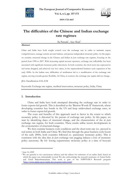
<strong>The</strong> <strong>difficulties</strong> <strong>of</strong> <strong>the</strong> <strong>Chinese</strong> <strong>and</strong> <strong>Indian</strong> <strong>exchange</strong><br />
<strong>rate</strong> <strong>regimes</strong><br />
Abstract<br />
Ila Patnaik 1 , Ajay Shah 2<br />
China <strong>and</strong> India have both sought control over <strong>the</strong> <strong>exchange</strong> <strong>rate</strong> in order to maintain export<br />
competitiveness, manage current account balance, <strong>and</strong> pursue independent monetary policy. In this paper,<br />
we examine structural change in <strong>the</strong> <strong>Chinese</strong> <strong>and</strong> <strong>Indian</strong> de facto <strong>exchange</strong> <strong>rate</strong> <strong>regimes</strong>, focusing on <strong>the</strong><br />
period from 1998 to 2007. With increasing capital account openness, <strong>exchange</strong> <strong>rate</strong> inflexibility has been<br />
associated with significant monetary policy distortions. In both countries, <strong>the</strong> short-term <strong>rate</strong> expressed in<br />
real terms dropped, <strong>and</strong> achieved very low values, in <strong>the</strong> unprecedented business cycle expansion <strong>of</strong> <strong>the</strong><br />
early 2000s. In <strong>the</strong> <strong>Indian</strong> case, <strong>difficulties</strong> <strong>of</strong> sterilisation led to a modification <strong>of</strong> <strong>the</strong> <strong>exchange</strong> <strong>rate</strong><br />
regime, moving towards greater flexibility. In China, in contrast, <strong>the</strong> <strong>exchange</strong> <strong>rate</strong> regime did not change.<br />
JEL Classification: E52, E58<br />
Keywords: Exchange <strong>rate</strong> regime, sterilised intervention, monetary policy, India, China.<br />
1. Introduction<br />
China <strong>and</strong> India have both attempted distorting <strong>the</strong> <strong>exchange</strong> <strong>rate</strong> in order to<br />
foster exports-led growth. This is described as <strong>the</strong> ‘Bretton Woods II’ framework, where<br />
developing countries buy bonds in <strong>the</strong> US <strong>and</strong> keep undervalued <strong>exchange</strong> <strong>rate</strong>s, in<br />
order to foster export-led growth.<br />
<strong>The</strong> costs <strong>and</strong> benefits <strong>of</strong> this approach need to factor in <strong>the</strong> extent to which<br />
monetary policy is distorted by <strong>the</strong> pursuit <strong>of</strong> <strong>exchange</strong> <strong>rate</strong> policy. In this paper, we<br />
start by identifying dates <strong>of</strong> structural change, <strong>and</strong> <strong>the</strong> characteristics <strong>of</strong> <strong>the</strong> de facto<br />
<strong>exchange</strong> <strong>rate</strong> regime, for both countries. <strong>The</strong>se results utilise recent developments in<br />
<strong>the</strong> econometrics <strong>of</strong> structural change.<br />
We <strong>the</strong>n examine business cycle conditions <strong>and</strong> <strong>the</strong> short-term <strong>rate</strong> (ex- pressed in<br />
real terms) in both India <strong>and</strong> China. We find that through <strong>the</strong> great business cycle boom<br />
<strong>of</strong> <strong>the</strong> early 2000s, both countries followed ex- pansionary monetary policy. This is<br />
consistent with <strong>the</strong> idea that de facto <strong>exchange</strong> <strong>rate</strong> pegging induces a loss <strong>of</strong> monetary<br />
policy autonomy. By fol- lowing expansionary monetary policy at a time <strong>of</strong> buoyant<br />
1 June 16, 2009<br />
2 We are g<strong>rate</strong>ful to two anonymous referees <strong>and</strong> <strong>the</strong> editors for criticisms <strong>of</strong> an earlier draft, based on<br />
which <strong>the</strong> paper was substantially revised. We also acknowledge <strong>the</strong> research assistance <strong>of</strong> Anmol Sethy<br />
<strong>and</strong> Vimal Balasubramaniam. This work is part <strong>of</strong> <strong>the</strong> NIPFP-DEA Research program<br />
(http://www.nipfp.org.in/nipfp-dea-program/index.html).<br />
Available online at http://eaces.liuc.it
158<br />
EJCE, vol.6, n. 1 (2009)<br />
business cycle conditions, in both countries, monetary policy contributed to<br />
exacerbating instability <strong>of</strong> GDP; it helped exacerbate both boom <strong>and</strong> bust.<br />
Capital flows <strong>and</strong> conditions on currency markets changed pr<strong>of</strong>oundly from late<br />
2007 onwards. Hence, this paper is primarily focused on <strong>the</strong> period from 1998 till 2007,<br />
<strong>the</strong> period where both countries were trying to use monetary policy to obtain <strong>exchange</strong><br />
<strong>rate</strong> undervaluation. <strong>The</strong>se <strong>difficulties</strong> need to be brought into <strong>the</strong> assessment <strong>of</strong> <strong>the</strong><br />
‘Bretton Woods II’ regime.<br />
2. <strong>The</strong> <strong>exchange</strong> <strong>rate</strong> regime<br />
An extensive literature suggests that both China <strong>and</strong> India have de facto pegged<br />
<strong>exchange</strong> <strong>rate</strong>s, where policy makers desire to influence <strong>the</strong> bilateral <strong>exchange</strong> <strong>rate</strong><br />
against <strong>the</strong> USD (Shah et al., 2005; Frankel, 2009; Patnaik, 2007).<br />
In India, according to <strong>the</strong> RBI (<strong>the</strong> <strong>Indian</strong> central bank), <strong>the</strong> rupee is a “market<br />
determined <strong>exchange</strong> <strong>rate</strong>”, in <strong>the</strong> sense that <strong>the</strong>re is a currency market <strong>and</strong> <strong>the</strong><br />
<strong>exchange</strong> <strong>rate</strong> is not administratively determined. India has clearly moved away from<br />
fixed <strong>exchange</strong> <strong>rate</strong>s. However, RBI actively trades on <strong>the</strong> market, with <strong>the</strong> goal <strong>of</strong><br />
“containing volatility”, <strong>and</strong> influencing <strong>the</strong> market price.<br />
Patnaik (2007) shows that <strong>the</strong> INR is de facto pegged to <strong>the</strong> USD. As is typical with<br />
such an <strong>exchange</strong> <strong>rate</strong> regime, <strong>the</strong> nominal INR/USD <strong>exchange</strong> <strong>rate</strong> has had low<br />
volatility, while all o<strong>the</strong>r measures <strong>of</strong> <strong>the</strong> <strong>exchange</strong> <strong>rate</strong> have been more volatile. Over<br />
<strong>the</strong> 1993-2006 period, <strong>the</strong> annualised volatility <strong>of</strong> <strong>the</strong> INR/USD was 4.2%. For a<br />
comparison, <strong>the</strong> annualised volatility <strong>of</strong> <strong>the</strong> USD/JPY <strong>rate</strong> was 11.6%.<br />
Figure 1 Comparing <strong>Chinese</strong> <strong>and</strong> <strong>Indian</strong> <strong>exchange</strong> <strong>rate</strong> movements<br />
China on <strong>the</strong> o<strong>the</strong>r h<strong>and</strong> is more open in discussing currency pegging. <strong>The</strong><br />
objective <strong>of</strong> monetary policy “is to maintain <strong>the</strong> stability <strong>of</strong> <strong>the</strong> value <strong>of</strong> <strong>the</strong> currency<br />
<strong>and</strong> <strong>the</strong>reby promote economic growth.”’ After being fixed to <strong>the</strong> US dollar for many<br />
years, China announced a shift away from a fixed <strong>rate</strong> to a basket peg in July 2005.<br />
However, <strong>the</strong> renminbi remained de facto pegged to <strong>the</strong> US dollar (Shah et al., 2005).<br />
2.1 Comparison <strong>of</strong> <strong>the</strong> level <strong>of</strong> <strong>the</strong> <strong>exchange</strong> <strong>rate</strong><br />
We embark on our comparison <strong>of</strong> <strong>the</strong> two <strong>exchange</strong> <strong>rate</strong> <strong>regimes</strong> by examining<br />
fluctuations <strong>of</strong> <strong>the</strong> bilateral <strong>exchange</strong> <strong>rate</strong> to <strong>the</strong> US dollar. This is shown in Figure 1. In<br />
Available online at http://eaces.liuc.it
<strong>The</strong> <strong>difficulties</strong> <strong>of</strong> <strong>the</strong> <strong>Chinese</strong> <strong>and</strong> <strong>Indian</strong> <strong>exchange</strong> <strong>rate</strong> <strong>regimes</strong><br />
159<br />
order to directly compare fluctuations <strong>of</strong> <strong>the</strong> INR <strong>and</strong> <strong>the</strong> CNY against <strong>the</strong> USD, <strong>the</strong><br />
Figure rescales <strong>the</strong> <strong>Chinese</strong> <strong>exchange</strong> <strong>rate</strong> to be identical to <strong>the</strong> rupee-dollar <strong>exchange</strong><br />
<strong>rate</strong> at <strong>the</strong> starting point <strong>of</strong> <strong>the</strong> graph.<br />
In <strong>the</strong>se units (i.e., rescaled to INR/USD <strong>exchange</strong> <strong>rate</strong> levels), both trajectories<br />
were similar, o<strong>the</strong>r than a substantial rupee depreciation from 2001 to 2002. <strong>The</strong> graph<br />
also visually conveys <strong>the</strong> greater flexibility <strong>of</strong> <strong>the</strong> bilateral rupee-dollar <strong>rate</strong> when<br />
compared with <strong>the</strong> yuan-dollar <strong>rate</strong>.<br />
A key concern <strong>of</strong> <strong>Chinese</strong> currency policy has been about <strong>the</strong> impact <strong>of</strong> <strong>the</strong> real<br />
<strong>exchange</strong> <strong>rate</strong> on exports. In <strong>the</strong> period from 2000 to 2007, <strong>the</strong> BIS real effective<br />
<strong>exchange</strong> <strong>rate</strong> for China showed a depreciation <strong>of</strong> 5%, while India showed an<br />
appreciation <strong>of</strong> 11.5%. Combined with <strong>the</strong> size <strong>of</strong> <strong>Chinese</strong> trade surpluses, especially<br />
with <strong>the</strong> US, <strong>the</strong> movement <strong>of</strong> <strong>the</strong> real <strong>exchange</strong> <strong>rate</strong> <strong>of</strong> <strong>the</strong> yuan has created a<br />
significant literature examining <strong>the</strong> issue <strong>of</strong> <strong>the</strong> undervaluation <strong>of</strong> <strong>the</strong> <strong>Chinese</strong> yuan<br />
(Goldstein <strong>and</strong> Lardy, 2008; Roubini, 2007; Goldstein, 2007). <strong>Indian</strong> policy makers have<br />
possibly favoured <strong>exchange</strong> <strong>rate</strong> depreciation owing to concerns about competitiveness<br />
<strong>of</strong> <strong>Indian</strong> exporters who compete with <strong>Chinese</strong> firms.<br />
Table 1 Volatility <strong>of</strong> <strong>the</strong> bilateral <strong>rate</strong> to <strong>the</strong> USD<br />
Year<br />
Annualised currency<br />
India<br />
volatility<br />
China<br />
1998<br />
1999<br />
5.568<br />
1.999<br />
0.856<br />
0.041<br />
2000 2.565 0.077<br />
2001<br />
2002<br />
2.055<br />
1.079<br />
0.047<br />
0.137<br />
2003<br />
2004<br />
2.147<br />
5.257<br />
0.055<br />
0.016<br />
2005 3.343 2.042<br />
2006<br />
2007<br />
3.518<br />
4.995<br />
0.749<br />
1.574<br />
2.2 Comparison <strong>of</strong> volatility <strong>of</strong> <strong>the</strong> <strong>exchange</strong> <strong>rate</strong> to <strong>the</strong> US dollar<br />
We examine <strong>the</strong> level <strong>and</strong> <strong>the</strong> time-series variation <strong>of</strong> <strong>the</strong> volatility <strong>of</strong> <strong>the</strong><br />
<strong>exchange</strong> <strong>rate</strong> to <strong>the</strong> US dollar in Table 1. This shows <strong>the</strong> volatility <strong>of</strong> <strong>the</strong> bilateral<br />
<strong>exchange</strong> <strong>rate</strong> (to <strong>the</strong> USD), for each year, for both China <strong>and</strong> India.<br />
In <strong>the</strong> <strong>Indian</strong> case, <strong>the</strong> volatility attained <strong>the</strong> highest values <strong>of</strong> roughly 5% per year<br />
in 1998 <strong>and</strong> 2007 with lower values seen in <strong>the</strong> intermediate years. In <strong>the</strong> <strong>Chinese</strong> case,<br />
<strong>the</strong> highest values seen were <strong>of</strong> 1.5% <strong>of</strong> 2%. This numerically restates <strong>the</strong> picture that is<br />
visible in Figure 1, <strong>of</strong> a less flexible <strong>Chinese</strong> <strong>exchange</strong> <strong>rate</strong> (expressed in US dollars).<br />
2.3 Extent to which appreciation against <strong>the</strong> USD was resisted<br />
A substantial decline in <strong>the</strong> US dollar took place from 31 January 2002 till 18<br />
March 2008. <strong>The</strong> US Fed calculates <strong>the</strong> ‘major currencies index’, an index <strong>of</strong> <strong>the</strong> US<br />
dollar against <strong>the</strong> major international currencies, all <strong>of</strong> which are floating <strong>exchange</strong> <strong>rate</strong>s.<br />
Over this period, this index fell from a value <strong>of</strong> 112.618 to a value <strong>of</strong> 69.263, a decline<br />
Available online at http://eaces.liuc.it
160<br />
EJCE, vol.6, n. 1 (2009)<br />
<strong>of</strong> 38.4%. Ordinary market forces would have gene<strong>rate</strong>d corresponding appreciations <strong>of</strong><br />
o<strong>the</strong>r currencies, when expressed against <strong>the</strong> dollar. <strong>The</strong> extent to which countries<br />
resisted appreciation against <strong>the</strong> dollar is a key factor explaining why some countries did<br />
not have significant appreciations. Table 2 compares some major currencies by <strong>the</strong>ir<br />
depreciation against <strong>the</strong> USD <strong>and</strong> also <strong>of</strong>fers an international comparison for <strong>the</strong><br />
annualised volatility <strong>of</strong> <strong>the</strong> bilateral <strong>exchange</strong> <strong>rate</strong> against <strong>the</strong> USD.<br />
Table 2 Depreciation <strong>of</strong> various currencies against <strong>the</strong> US dollar between 31 January 2002 <strong>and</strong> 18 March 2008<br />
Rank Country or area currency<br />
Depreciation Volatility<br />
(Percent) (Annualised)<br />
1 New Zeal<strong>and</strong> New Zeal<strong>and</strong> Dollar -48.44 11.94<br />
2 Eurozone Euro -45.43 8.74<br />
3 Denmark Danish Krone -45.22 8.76<br />
4 Australia Australian dollar -45.21 10.29<br />
5 Sweden Swedish Krona -43.95 10.11<br />
6 Norway Norwegian Krone -43.84 11.08<br />
7 Switzerl<strong>and</strong> Swiss franc -42.38 9.66<br />
8 US major currencies index -38.40<br />
9 Canada Canadian dollar -37.53 8.00<br />
10 South Africa R<strong>and</strong> -31.21 16.76<br />
11 Great Britain Pound -29.97 8.11<br />
12 Thail<strong>and</strong> Thai baht -29.41 7.49<br />
13 Brazil Real -29.33 15.49<br />
14 Japan Yen -26.57 9.47<br />
15 Singapore Singapore dollar -24.93 4.05<br />
16 South-Korea Won -23.47 6.77<br />
17 India <strong>Indian</strong> rupee -17.20 3.83<br />
18 Malaysia Ringgit -17.01 2.48<br />
19 China Yuan-Renminbi -14.46 1.19<br />
20 Taiwan Taiwan dollar -12.23 3.85<br />
21 Hong Kong Hong Kong dollar -0.38 0.55<br />
22 Sri Lanka Rupee 14.96 4.15<br />
23 Mexico Mexican peso 17.02 6.78<br />
24 Venezuela Venezuelan bolivar 179.32 19.45<br />
While floating <strong>exchange</strong> <strong>rate</strong>s had an appreciation against <strong>the</strong> dollar <strong>of</strong> 38.4%,<br />
India (ranked 17th in this list), had an appreciation <strong>of</strong> 17.19% <strong>and</strong> China (ranked 19th)<br />
had an appreciation <strong>of</strong> 14.46%. Only three currencies - from rank 22 to rank 24 -<br />
showed a depreciation against <strong>the</strong> US dollar in this period. Of <strong>the</strong>se, two countries (Sri<br />
Lanka <strong>and</strong> Venezuela) were under particularly adverse political conditions.<br />
Available online at http://eaces.liuc.it
<strong>The</strong> <strong>difficulties</strong> <strong>of</strong> <strong>the</strong> <strong>Chinese</strong> <strong>and</strong> <strong>Indian</strong> <strong>exchange</strong> <strong>rate</strong> <strong>regimes</strong><br />
161<br />
Ranked by rigidity <strong>of</strong> <strong>the</strong> bilateral <strong>exchange</strong> <strong>rate</strong> against <strong>the</strong> USD, <strong>the</strong> <strong>Chinese</strong><br />
Yuan is at rank 2 <strong>and</strong> <strong>the</strong> <strong>Indian</strong> rupee is at rank 4 in this list. This evidence suggests<br />
that both India <strong>and</strong> China were de facto pegs to <strong>the</strong> US dollar, with very low currency<br />
flexibility by international st<strong>and</strong>ards.<br />
2.4 Fine structure <strong>of</strong> <strong>the</strong> <strong>exchange</strong> <strong>rate</strong> regime<br />
In <strong>the</strong> last decade, <strong>the</strong> literature has revealed that <strong>the</strong> de jure <strong>exchange</strong> <strong>rate</strong> regime<br />
in operation in many countries that is announced by <strong>the</strong> central bank differs from <strong>the</strong> de<br />
facto regime in operation. This has motivated a small literature on data-driven methods<br />
for <strong>the</strong> classification <strong>of</strong> <strong>exchange</strong> <strong>rate</strong> <strong>regimes</strong> (see e.g., Reinhart <strong>and</strong> Rog<strong>of</strong>f, 2004;<br />
Levy-Yeyati <strong>and</strong> Sturzenegger, 2003; Calvo <strong>and</strong> Reinhart, 2002). This literature has<br />
attempted to create datasets identifying <strong>the</strong> <strong>exchange</strong> <strong>rate</strong> regime in operation for all<br />
countries in recent decades, using a variety <strong>of</strong> alternative algorithms. While <strong>the</strong>se<br />
databases are useful for many applications, <strong>the</strong>y have limited usefulness in measuring <strong>the</strong><br />
fine structure <strong>of</strong> intermediate <strong>regimes</strong>. As an example, <strong>the</strong> Reinhart <strong>and</strong> Rog<strong>of</strong>f<br />
classification sees <strong>the</strong> <strong>Indian</strong> rupee as a single <strong>exchange</strong> <strong>rate</strong> regime from 1993 onwards.<br />
As <strong>the</strong> evidence ahead shows, <strong>the</strong>re is a fine structure in <strong>the</strong> post-1993 period which<br />
yields fresh insights into <strong>the</strong> causes <strong>and</strong> consequences <strong>of</strong> <strong>the</strong> <strong>exchange</strong> <strong>rate</strong> regime <strong>and</strong><br />
monetary policy framework.<br />
A valuable tool for underst<strong>and</strong>ing <strong>the</strong> de facto <strong>exchange</strong> <strong>rate</strong> regime in operation is<br />
a linear regression model based on cross-currency <strong>exchange</strong> <strong>rate</strong>s (with respect to a<br />
suitable numeraire). Used at least since Haldane <strong>and</strong> Hall (1991), this model was<br />
popularized by Frankel <strong>and</strong> Wei (1994) (<strong>and</strong> is hence also called Frankel-Wei model).<br />
Recent applications <strong>of</strong> this estimation st<strong>rate</strong>gy include B´enassy-Qu´er´e et al. (2006),<br />
Shah et al. (2005) <strong>and</strong> Frankel <strong>and</strong> Wei (2007). In this approach, an independent<br />
currency, such as <strong>the</strong> Swiss Franc (CHF), is chosen as an arbitrary ‘numeraire’. If<br />
estimation involving <strong>the</strong> <strong>Indian</strong> rupee (INR) is desired, <strong>the</strong> model estimated is:<br />
This regression picks up <strong>the</strong> extent to which <strong>the</strong> INR/CHF <strong>rate</strong> fluctuates in<br />
response to fluctuations in <strong>the</strong> USD/CHF <strong>rate</strong>. If <strong>the</strong>re is pegging to <strong>the</strong> USD, <strong>the</strong>n<br />
fluctuations in <strong>the</strong> JPY <strong>and</strong> DEM will be irrelevant, <strong>and</strong> we will observe β3 = β4 = 0<br />
while β2 = 1. If <strong>the</strong>re is no pegging, <strong>the</strong>n all <strong>the</strong> three betas will be different from 0. <strong>The</strong><br />
R 2 <strong>of</strong> this regression is also <strong>of</strong> interest; values near 1 would suggest reduced <strong>exchange</strong><br />
<strong>rate</strong> flexibility.<br />
To underst<strong>and</strong> <strong>the</strong> de facto <strong>exchange</strong> <strong>rate</strong> regime in a given country in a given time<br />
period, researchers <strong>and</strong> practitioners can easily fit this regression model to a given data<br />
window, or use rolling data windows. However, such a st<strong>rate</strong>gy lacks a formal inferential<br />
framework for determining changes in <strong>the</strong> <strong>regimes</strong>. This has motivated an extension <strong>of</strong><br />
<strong>the</strong> econometrics <strong>of</strong> structural change for <strong>the</strong> purpose <strong>of</strong> analysing structural change in<br />
<strong>the</strong> Frankel-Wei model (Zeileis et al., 2008). This involves extending <strong>the</strong> familiar Perron-<br />
Bai methodology (Bai <strong>and</strong> Perron, 2003) for identifying <strong>the</strong> dates <strong>of</strong> structural change in<br />
an OLS regression. Through this, dates <strong>of</strong> structural change in <strong>the</strong> <strong>exchange</strong> <strong>rate</strong> regime<br />
are identified. We focus on <strong>the</strong> period after 1994, <strong>and</strong> utilise weekly changes in <strong>exchange</strong><br />
<strong>rate</strong>s for <strong>the</strong>se estimations. Values shown in brackets are t statistics.<br />
Available online at http://eaces.liuc.it
162<br />
EJCE, vol.6, n. 1 (2009)<br />
Table 3 China’s de facto <strong>exchange</strong> <strong>rate</strong> regime<br />
Period USD JPY EUR GBP σ e R 2<br />
15 Apr ’94 - 22 Jul ’05 1.006<br />
(215.9)<br />
22 Jul ’05 - 17 Apr ’09 0.949<br />
(56.8)<br />
-0.003<br />
(-1.0)<br />
0.008<br />
(0.6)<br />
0.015<br />
(1.47)<br />
0.062<br />
(2.3)<br />
-0.008<br />
(-1.4)<br />
0.002<br />
(0.1)<br />
0.113 0.994<br />
0.243 0.974<br />
Table 3 shows <strong>the</strong> results <strong>of</strong> this estimation st<strong>rate</strong>gy for <strong>the</strong> <strong>Chinese</strong> Renminbi. It<br />
finds that <strong>the</strong> first period runs from 15 April 1994 till 22 July 2005. This is a simple<br />
USD peg, with a coefficient <strong>of</strong> 1 for <strong>the</strong> USD, zero coefficients on all o<strong>the</strong>r currencies, a<br />
residual st<strong>and</strong>ard deviation <strong>of</strong> 0.113 <strong>and</strong> an R 2 <strong>of</strong> 0.994. From 22 July 2005 till 17 April<br />
2009, a single sub-period <strong>of</strong> <strong>the</strong> <strong>exchange</strong> <strong>rate</strong> regime holds.<br />
In some respects, this result agrees with <strong>of</strong>ficial statements <strong>and</strong> a simple visual<br />
examination <strong>of</strong> <strong>the</strong> <strong>exchange</strong> <strong>rate</strong>. <strong>The</strong> break date <strong>of</strong> 22 July 2005 that is derived from<br />
<strong>the</strong> econometrics is consistent with that announced by <strong>the</strong> authorities. In <strong>the</strong>se respects,<br />
<strong>the</strong> results for China help us see that <strong>the</strong> econometric analysis is broadly on <strong>the</strong> right<br />
track.<br />
At <strong>the</strong> same time, <strong>the</strong>re is something important in <strong>the</strong> fact that after 22 July 2005,<br />
no fur<strong>the</strong>r structural change is announced. This contradicts a variety <strong>of</strong> <strong>of</strong>ficial claims<br />
which have been made about <strong>the</strong> evolution <strong>of</strong> <strong>the</strong> <strong>exchange</strong> <strong>rate</strong> away from dollar<br />
pegging towards a basket peg, <strong>and</strong> towards greater <strong>exchange</strong> <strong>rate</strong> flexibility.<br />
<strong>The</strong> econometrics suggests that remarkably little has changed about <strong>the</strong> actual<br />
<strong>exchange</strong> <strong>rate</strong> regime in operation when compared with <strong>the</strong> previous regime. <strong>The</strong> USD<br />
coefficient has dropped to 0.949. A statistically significant Euro coefficient has emerged,<br />
with a small value <strong>of</strong> 0.06 where <strong>the</strong> null hypo<strong>the</strong>sis <strong>of</strong> 0 can be rejected. <strong>The</strong> residual<br />
st<strong>and</strong>ard deviation has more than doubled to 0.243. But <strong>the</strong> R 2 has dropped only slightly<br />
to 0.974. While <strong>the</strong>re was more <strong>exchange</strong> <strong>rate</strong> flexibility in this period, <strong>the</strong> change in <strong>the</strong><br />
<strong>exchange</strong> <strong>rate</strong> regime was extremely small.<br />
While <strong>the</strong> dating methodology <strong>of</strong> Zeileis et al. (2008) reports a structural break on<br />
22 July 2005, <strong>the</strong> difference that came about in <strong>the</strong> <strong>exchange</strong> <strong>rate</strong> regime is small. <strong>The</strong><br />
euclidian distance between <strong>the</strong> vector <strong>of</strong> slopes before <strong>and</strong> after works out to just 0.075.<br />
In India, when <strong>the</strong> rupee began its life as a ‘market determined <strong>exchange</strong> <strong>rate</strong>’ in<br />
March 1993, for <strong>the</strong> first two years, <strong>the</strong> <strong>exchange</strong> <strong>rate</strong> regime was actually almost a fixed<br />
<strong>exchange</strong> <strong>rate</strong> to <strong>the</strong> USD. <strong>The</strong> USD coefficient was 0.967 <strong>and</strong> <strong>the</strong> only o<strong>the</strong>r<br />
statistically significant coefficient was <strong>the</strong> JPY at 0.028. <strong>The</strong> residual st<strong>and</strong>ard deviation<br />
was 0.164 <strong>and</strong> <strong>the</strong> R 2 was 0.9887. This was greater <strong>exchange</strong> <strong>rate</strong> inflexibility than that<br />
found in China after July 2005.<br />
Available online at http://eaces.liuc.it
<strong>The</strong> <strong>difficulties</strong> <strong>of</strong> <strong>the</strong> <strong>Chinese</strong> <strong>and</strong> <strong>Indian</strong> <strong>exchange</strong> <strong>rate</strong> <strong>regimes</strong><br />
163<br />
Table 4 India’s de facto <strong>exchange</strong> <strong>rate</strong> regime<br />
Period USD JPY EUR GBP σ e R 2<br />
19 Mar ’93 - 3 Mar ’95 0.967 0.028 0.012 0.028 0.164 0.989<br />
(58.3) (2.0) (0.4) (1.3)<br />
10 Mar ’95 - 21 Aug ’98 0.943 0.067 -0.026 0.042 0.937 0.729<br />
(12.8) (1.4) (-0.2) (0.6)<br />
28 Aug ’98 - 19 Mar ’04 0.993 0.010 0.098 -0.003 0.277 0.969<br />
(61.7) (1.0) (2.9) (-0.2)<br />
26 Mar ’04 - 17 Apr ’09 0.734 0.050 0.440 0.086 0.853 0.721<br />
(14.5) (1.2) (5.0) (2.0)<br />
In <strong>the</strong> period <strong>of</strong> <strong>the</strong> Asian crisis, <strong>the</strong>re was a dramatic change in flexibility in <strong>the</strong><br />
<strong>Indian</strong> <strong>exchange</strong> <strong>rate</strong> regime. <strong>The</strong> residual st<strong>and</strong>ard deviation rose to 0.937, <strong>and</strong> <strong>the</strong> R 2<br />
dropped to 0.729. However, <strong>the</strong> only significant coefficient in <strong>the</strong> regression was <strong>the</strong><br />
USD with a value <strong>of</strong> 0.943 which is not much different from 1. This was, hence, a<br />
period <strong>of</strong> pegging to <strong>the</strong> USD, with significant flexibility.<br />
After this, India returned to USD pegging. From 28 August 1998 till 19 March<br />
2004, <strong>the</strong> USD coefficient went back to 0.993. <strong>The</strong> only o<strong>the</strong>r significant coefficient was<br />
for <strong>the</strong> Euro, with a value <strong>of</strong> 0.098. <strong>The</strong> residual st<strong>and</strong>ard deviation went back down to<br />
0.277 <strong>and</strong> <strong>the</strong> R 2 rose to 0.969. In this period, <strong>the</strong> <strong>exchange</strong> <strong>rate</strong> regime in India was<br />
similar to that found in China after July 2005.<br />
In <strong>the</strong> last period, India returned to significant <strong>exchange</strong> <strong>rate</strong> flexibility. <strong>The</strong> USD<br />
coefficient dropped to 0.734. Coefficients for <strong>the</strong> Euro <strong>and</strong> <strong>the</strong> Pound were statistically<br />
significant, <strong>and</strong> <strong>the</strong> Euro coefficient was economically significant at 0.44. <strong>The</strong> residual<br />
st<strong>and</strong>ard deviation rose to 0.853 <strong>and</strong> <strong>the</strong> R 2 dropped to 0.721. <strong>The</strong> change in <strong>the</strong><br />
<strong>exchange</strong> <strong>rate</strong> regime which took place in March 2004 was both statistically significant<br />
<strong>and</strong> economically significant. <strong>The</strong> euclidian distance between <strong>the</strong> vector <strong>of</strong> slopes that<br />
prevailed before <strong>and</strong> after this date works out to 0.44, which is six times bigger than that<br />
associated with <strong>the</strong> <strong>Chinese</strong> <strong>exchange</strong> <strong>rate</strong> regime reform <strong>of</strong> July 2005.<br />
3. Capital controls<br />
<strong>The</strong> Chinn-Ito measure <strong>of</strong> de jure capital controls (Chinn <strong>and</strong> Ito, 2008) shows that<br />
both countries have had substantial capital controls. For both China <strong>and</strong> India, <strong>the</strong><br />
Chinn-Ito measure stagnated at -1.13 from 1970 till 2007.<br />
This was in sharp contrast with <strong>the</strong> substantial scale <strong>of</strong> de jure capital account<br />
decontrol which took place worldwide. Figure 2 shows <strong>the</strong> kernel density plot <strong>of</strong> <strong>the</strong><br />
Chinn-Ito measure across all countries. In both years, <strong>the</strong> density is bimodal, with a<br />
cluster <strong>of</strong> countries with largely open capital accounts <strong>and</strong> a cluster <strong>of</strong> countries with<br />
largely closed capital accounts. In 1970, <strong>the</strong> value <strong>of</strong> -1.13 was close to <strong>the</strong> mode. From<br />
1970 to 2007, many countries mig<strong>rate</strong>d away from capital controls. China <strong>and</strong> India<br />
were not among <strong>the</strong>se.<br />
<strong>The</strong> world mean Chinn-Ito score went from -0.4 in 1970 to +0.5 in 2007. In Asia,<br />
<strong>the</strong> Chinn-Ito score averaged -0.32 in 1970. It went up to 0.43 in 2007. Emerging<br />
markets averaged -0.38 in 1970; this went up to 0.59 in 2007. Finally, <strong>the</strong> G-20 countries<br />
Available online at http://eaces.liuc.it
164<br />
EJCE, vol.6, n. 1 (2009)<br />
experienced an evolution <strong>of</strong> <strong>the</strong> average Chinn-Ito score from 0.03 in 1970 to 1.52 in<br />
2007. Hence, whe<strong>the</strong>r China <strong>and</strong> India are compared against <strong>the</strong> world average, against<br />
Asia, against emerging markets or against G-20 members, <strong>the</strong> lack <strong>of</strong> de jure capital<br />
account liberalisation in <strong>the</strong>se countries st<strong>and</strong>s out when compared with <strong>the</strong><br />
developments worldwide.<br />
Figure 2 Density <strong>of</strong> <strong>the</strong> Chinn-Ito measure: comparing 1970 vs. 2007<br />
At first blush, a consistent monetary policy regime requires capital controls when<br />
<strong>exchange</strong> <strong>rate</strong> inflexibility is present, so as to ensure autonomy <strong>of</strong> domestic monetary<br />
policy. Hence, <strong>the</strong> exceptional use <strong>of</strong> strong de jure capital controls by China <strong>and</strong> India<br />
(by international st<strong>and</strong>ards) is consistent with <strong>the</strong> exceptional <strong>exchange</strong> <strong>rate</strong> inflexibility<br />
in <strong>the</strong>se countries (by international st<strong>and</strong>ards).<br />
<strong>The</strong> difficulty with this lies in <strong>the</strong> distinction between de jure <strong>and</strong> de facto capital<br />
controls. Both countries have experimented with a controlled opening <strong>of</strong> <strong>the</strong> capital<br />
account. This has brought about elements <strong>of</strong> openness. Both countries have pursued<br />
trade integration, <strong>and</strong> have witnessed a massive expansion in <strong>the</strong> size <strong>of</strong> <strong>the</strong> current<br />
account relative to GDP. Accompanying this is an enlarged set <strong>of</strong> opportunities for<br />
evading capital controls through misinvoicing. <strong>The</strong> international experience suggests<br />
that over time, <strong>the</strong> effectiveness <strong>of</strong> capital controls is diminished, as economic agents<br />
underst<strong>and</strong> how to evade <strong>the</strong>m.<br />
If capital controls were binding, <strong>the</strong>n both countries would enjoy a consistent<br />
monetary policy regime, with a closed capital account <strong>and</strong> <strong>exchange</strong> <strong>rate</strong> rigidity not<br />
interfering with autonomy <strong>of</strong> monetary policy. To <strong>the</strong> extent that <strong>the</strong>re is de facto<br />
openness <strong>of</strong> <strong>the</strong> capital account, both countries would find that <strong>exchange</strong> <strong>rate</strong><br />
distortions would yield monetary policy distortions.<br />
Available online at http://eaces.liuc.it
<strong>The</strong> <strong>difficulties</strong> <strong>of</strong> <strong>the</strong> <strong>Chinese</strong> <strong>and</strong> <strong>Indian</strong> <strong>exchange</strong> <strong>rate</strong> <strong>regimes</strong><br />
165<br />
4. <strong>The</strong> implementation <strong>of</strong> <strong>the</strong> <strong>exchange</strong> <strong>rate</strong> regime<br />
In both countries, currency pegging has been achieved through intervention in <strong>the</strong><br />
foreign <strong>exchange</strong> market leading to a large buildup <strong>of</strong> reserves in both countries. To<br />
avoid <strong>the</strong> inflationary impact <strong>of</strong> this intervention, <strong>the</strong> central banks <strong>of</strong> both India <strong>and</strong><br />
China have attempted to sterilise this intervention (Lafrance, 2008; Aizenman <strong>and</strong> Glick,<br />
2008). However, in recent years, as is acknowledged by <strong>the</strong> central bank in China, <strong>the</strong><br />
People’s Bank <strong>of</strong> China (PBoC) <strong>and</strong> documented by a number <strong>of</strong> studies, it was<br />
becoming increasingly difficult to sterilise its intervention in China (McKinnon <strong>and</strong><br />
Schnabl, 2008; Prasad, 2008; Kwan, 2006; Hannoun, 2007).<br />
<strong>The</strong> People’s Bank <strong>of</strong> China focussed on addressing <strong>the</strong>se <strong>difficulties</strong> implemented<br />
a mix <strong>of</strong> measures such as open market operations, increase in reserve<br />
requirements <strong>and</strong> targetted issue <strong>of</strong> central bank bills <strong>the</strong>re were meant to sterilise <strong>the</strong><br />
liquidity supplied as a result <strong>of</strong> foreign <strong>exchange</strong> purchases.<br />
Figure 3 Rising foreign <strong>exchange</strong> reserves<br />
Figure 3 shows China’s sharply rising reserves. As capital inflows <strong>and</strong> current<br />
account surpluses grew, currency pegging required larger intervention <strong>and</strong> hence an<br />
increasing pace <strong>of</strong> reserve accumulation. <strong>The</strong> pace <strong>of</strong> reserves accumulation steadily<br />
escalated. Reserves grew by 0.59% per month between Mar 1997 <strong>and</strong> May 2001; <strong>the</strong>n<br />
<strong>the</strong>y grew by 1.37% per month between Jun 2001 <strong>and</strong> Oct 2002; <strong>the</strong>n <strong>the</strong>y grew by<br />
more than 2.5% per month from Nov 2002 until <strong>the</strong> global financial crisis.<br />
<strong>The</strong> size <strong>of</strong> foreign <strong>exchange</strong> reserves in China <strong>and</strong> India must be looked at in <strong>the</strong><br />
context <strong>of</strong> <strong>the</strong> size <strong>of</strong> <strong>the</strong> economy. <strong>Chinese</strong> GDP is much bigger than <strong>Indian</strong> GDP. In<br />
both countries, sterilisation involves selling government bonds which are largely bought<br />
by banks. In China, bank deposits are 150% <strong>of</strong> GDP while in India, <strong>the</strong>y are only 50%<br />
<strong>of</strong> GDP. Hence, <strong>the</strong> scale <strong>of</strong> sterilisation in China can be bigger than that seen in India.<br />
Prasad (2007) points out that in China household <strong>and</strong> corpo<strong>rate</strong> savings <strong>rate</strong>s are<br />
very high. Financial system repression has meant that <strong>the</strong>re are few alternatives to<br />
funnelling <strong>the</strong>se savings into deposits in <strong>the</strong> state-owned banking system. With <strong>the</strong> high<br />
growth <strong>rate</strong> <strong>of</strong> GDP growth <strong>and</strong> investment <strong>and</strong> fears <strong>of</strong> overheating, banks are under<br />
Available online at http://eaces.liuc.it
166<br />
EJCE, vol.6, n. 1 (2009)<br />
pressure to reduce credit growth. This has made banks flush with liquidity. Banks hold<br />
excess reserves with <strong>the</strong> PBC even though bank reserve requirements have been raised<br />
<strong>and</strong> returns on excess reserves reduced sharply. Capital adequacy norms <strong>of</strong> <strong>the</strong> PBC also<br />
increase <strong>the</strong> incentive <strong>of</strong> banks to hold goverment/PBC bills as <strong>the</strong>y carry zero capital<br />
requirement, while corpo<strong>rate</strong> bonds carry a capital requirement <strong>of</strong> hundred percent.<br />
<strong>The</strong>re are thus many reasons for banks to want to hold government bills at relatively<br />
low <strong>rate</strong>s.<br />
Figure 4 Reserves to GDP ratio<br />
In 2003, China ran out <strong>of</strong> government bonds for <strong>the</strong> purpose <strong>of</strong> sterilisation. 3<br />
<strong>The</strong>ir response was to initiate bills sold by <strong>the</strong> PBOC, called ‘PBOC Bills’, from April<br />
2003 onwards.<br />
This differs from <strong>the</strong> <strong>Indian</strong> setting, where <strong>the</strong> RBI Act does not permit RBI to<br />
issue bonds. Hence, when <strong>the</strong> <strong>Indian</strong> equivalent <strong>of</strong> PBOC bills was put into place in<br />
2004, this involved sale <strong>of</strong> ‘MSS bonds’ by RBI as an agent <strong>of</strong> MOF. <strong>The</strong> fiscal cost <strong>of</strong><br />
MSS bonds is clearly placed upon <strong>the</strong> exchequer in India, while in China, it only shows<br />
up as reduced dividend payments by <strong>the</strong> central bank.<br />
In India, <strong>the</strong> extent <strong>of</strong> sterilisation changed pr<strong>of</strong>oundly once MSS came into play.<br />
This partly reflects <strong>the</strong> fact that once <strong>the</strong> costs <strong>of</strong> <strong>the</strong> pegged <strong>exchange</strong> <strong>rate</strong> became part<br />
<strong>of</strong> <strong>the</strong> budgeting process, <strong>the</strong>y were subject to greater political scrutiny <strong>of</strong> <strong>the</strong> budget<br />
process. In contrast, in China, <strong>the</strong>re has been no restraint impeding a massive scale <strong>of</strong><br />
issuance <strong>of</strong> PBOC bills. In India, <strong>the</strong>re is a link between <strong>the</strong> event <strong>of</strong> running out <strong>of</strong><br />
bonds for sterilisation (December 2003) <strong>and</strong> <strong>the</strong> structural break in <strong>the</strong> <strong>exchange</strong> <strong>rate</strong><br />
regime (March 2004).<br />
Initially, PBOC bills were <strong>of</strong> three month maturity. However, <strong>the</strong> issuance shifted<br />
to one-year maturity. This involves somewhat higher costs reflecting <strong>the</strong> fact that oneyear<br />
bonds have a higher <strong>rate</strong> than three-month bonds. <strong>The</strong> massive pace <strong>of</strong> issuance<br />
led to higher <strong>rate</strong>s on PBOC bills. In August 2006, this <strong>rate</strong> stood at 2.796, a rise <strong>of</strong> 0.9<br />
percentage points over <strong>the</strong> year.<br />
As <strong>the</strong> <strong>Chinese</strong> reserves accumulation proceeded, despite <strong>the</strong> low interest <strong>rate</strong>s <strong>the</strong><br />
issuance <strong>of</strong> PBOC bills led to high fiscal costs <strong>and</strong> <strong>the</strong> difficulty that high interest <strong>rate</strong>s<br />
3 Source: China in Transition by Chi Hung Kwan, August 2006.<br />
Available online at http://eaces.liuc.it
<strong>The</strong> <strong>difficulties</strong> <strong>of</strong> <strong>the</strong> <strong>Chinese</strong> <strong>and</strong> <strong>Indian</strong> <strong>exchange</strong> <strong>rate</strong> <strong>regimes</strong><br />
167<br />
would suck in fur<strong>the</strong>r capital flows. From May 2006 onwards, PBOC bills have been<br />
issued under a ‘targeted issue’ scheme, where specific commercial banks are forced to<br />
buy specific quantities <strong>of</strong> PBOC bills at an interest <strong>rate</strong> below <strong>the</strong> market interest <strong>rate</strong>.<br />
For instance, on June 14, <strong>the</strong> PBC made a targeted issue <strong>of</strong> one-year maturity bills worth<br />
100 billion yuan at a yield <strong>of</strong> 2.1138 per cent, 0.4 per cent lower than <strong>the</strong> <strong>the</strong>n prevailing<br />
market <strong>rate</strong>. Of <strong>the</strong> PBC bills issued, 42 billion yuan were forced on China Construction<br />
Bank, 30 billion yuan on Agricultural Bank <strong>of</strong> China, 12 billion yuan on Industrial <strong>and</strong><br />
Commercial Bank <strong>of</strong> China, 10 billion yuan on Bank <strong>of</strong> Communications, <strong>and</strong> <strong>the</strong><br />
remaining 6 billion yuan on o<strong>the</strong>rs.<br />
To deal with rising <strong>difficulties</strong> PBOC raised reserve requirements by a cumulative<br />
3 percentage points on five occasions in 2008, freezing 70 percent <strong>of</strong> <strong>the</strong><br />
increased liquidity as a result <strong>of</strong> foreign <strong>exchange</strong> purchases PBOC (2009).<br />
In terms <strong>of</strong> <strong>the</strong> evolution <strong>of</strong> <strong>the</strong> <strong>Indian</strong> <strong>exchange</strong> <strong>rate</strong> regime, <strong>the</strong> period <strong>of</strong><br />
successful sterilised intervention aligns well with <strong>the</strong> sub-period <strong>of</strong> <strong>the</strong> <strong>exchange</strong> <strong>rate</strong><br />
regime drawn from Table 4, from 28 August 1998 to 19 March 2004, where <strong>the</strong>re was a<br />
tight peg to <strong>the</strong> US dollar with an R 2 <strong>of</strong> 0.969.<br />
In late 2003, RBI ran out <strong>of</strong> bonds for sterilisation. A short while later, <strong>the</strong><br />
<strong>exchange</strong> <strong>rate</strong> regime changed from 26 March 2004 onwards to have greater <strong>exchange</strong><br />
<strong>rate</strong> flexibility. In contrast, in China’s case, no comparable modification <strong>of</strong> <strong>the</strong> <strong>exchange</strong><br />
<strong>rate</strong> regime took place.<br />
5. <strong>The</strong> implications <strong>of</strong> <strong>the</strong> <strong>exchange</strong> <strong>rate</strong> regime for monetary policy<br />
When <strong>the</strong> capital account is perfectly open, <strong>exchange</strong> <strong>rate</strong> policy inevitably<br />
involves distorted interest <strong>rate</strong>s. In <strong>the</strong> case <strong>of</strong> China <strong>and</strong> India, while capital controls<br />
are very restrictive at a de jure level, <strong>the</strong>re is significant openness at a de facto level. As a<br />
consequence, attempts at <strong>exchange</strong> <strong>rate</strong> pegging have come at <strong>the</strong> cost <strong>of</strong> monetary<br />
policy autonomy.<br />
Capital flows generally tend to be procyclical. As a consequence, when business<br />
cycle conditions are good, capital tends to come into <strong>the</strong> country. If <strong>the</strong> central bank<br />
tries to prevent appreciation by purchasing dollars, this leads to low short term interest<br />
<strong>rate</strong>. Conversely, if <strong>exchange</strong> <strong>rate</strong> depreciation is prevented by <strong>the</strong> central bank when<br />
times are difficult, this requires an ‘interest <strong>rate</strong> defence’, i.e. high interest <strong>rate</strong>s when<br />
times are bad.<br />
In <strong>the</strong> <strong>Indian</strong> case, <strong>the</strong> experience is summarised by comparing Figure 5 which<br />
uses quarterly GDP growth to show business cycle conditions, <strong>and</strong> Figure 6 which<br />
shows a measure <strong>of</strong> <strong>the</strong> policy <strong>rate</strong> expressed in real terms. 4<br />
<strong>The</strong> period over which India had highly restricted <strong>exchange</strong> <strong>rate</strong> flexibility ran<br />
from August 1998 to March 2004. Late in this period, business cycle conditions<br />
improved dramatically, with quarterly GDP growth going from 2% on a year-on-year<br />
basis to over 10%. In this period, capital came into <strong>the</strong> country. Exchange <strong>rate</strong> pegging<br />
meant that dollars had to be purchased. With incomplete sterilisation, interest <strong>rate</strong>s in<br />
<strong>the</strong> domestic economy dropped sharply. <strong>The</strong> real <strong>rate</strong> fell from +3% to -4%: a 700 bps<br />
monetary policy easing at a time <strong>of</strong> an unprecedented business cycle expansion. <strong>The</strong><br />
change in <strong>the</strong> <strong>exchange</strong> <strong>rate</strong> regime in 2004 helped to improve monetary policy<br />
autonomy, <strong>and</strong> <strong>the</strong> real <strong>rate</strong> went up to 0. This was still a very low level <strong>of</strong> <strong>the</strong> real <strong>rate</strong><br />
4 <strong>The</strong> methodology for Figure 6 is based on Bhattacharya et al. (2008).<br />
Available online at http://eaces.liuc.it
168<br />
EJCE, vol.6, n. 1 (2009)<br />
considering that India was experiencing unprecedentedly benign business cycle<br />
conditions.<br />
Turning to China, Figure 7 shows a measure <strong>of</strong> <strong>Chinese</strong> business cycle conditions:<br />
<strong>the</strong> quarterly GDP growth. This shows an enormous boom in GDP growth from 2002<br />
onwards till 2007. Juxtaposing this against Figure 8, which shows <strong>the</strong> 90-day treasury bill<br />
<strong>rate</strong> (expressed in real terms), we see that from 2002 till early 2008, <strong>the</strong> real <strong>rate</strong> dropped<br />
by an enormous 800 basis points. This suggests that in good times, monetary policy was<br />
expansionary. This is consistent with <strong>the</strong> idea that <strong>exchange</strong> <strong>rate</strong> pegging converts <strong>the</strong><br />
pro-cyclicality <strong>of</strong> capital flows into pro-cyclicality <strong>of</strong> monetary policy.<br />
Figure 5 <strong>Indian</strong> quarterly GDP growth<br />
Figure 6 <strong>Indian</strong> real <strong>rate</strong><br />
Available online at http://eaces.liuc.it
<strong>The</strong> <strong>difficulties</strong> <strong>of</strong> <strong>the</strong> <strong>Chinese</strong> <strong>and</strong> <strong>Indian</strong> <strong>exchange</strong> <strong>rate</strong> <strong>regimes</strong><br />
169<br />
Figure 7 <strong>Chinese</strong> business cycle conditions (quarterly GDP growth)<br />
<strong>The</strong> use <strong>of</strong> loose monetary policy at a time <strong>of</strong> an unprecedented business cycle<br />
expansion, in both countries, helped induce an acceleration <strong>of</strong> inflation <strong>and</strong> an asset<br />
price boom.<br />
Figure 9 shows <strong>the</strong> time-series <strong>of</strong> <strong>the</strong> <strong>Indian</strong> CPI inflation. Through <strong>the</strong> decade <strong>of</strong><br />
<strong>the</strong> 1990s, <strong>the</strong>re was a prolonged effort in India to bring down inflation. By <strong>the</strong> end <strong>of</strong><br />
<strong>the</strong> 1990s, CPI inflation had dropped to near-zero levels. <strong>The</strong> persistent use <strong>of</strong> low<br />
policy <strong>rate</strong>s helped induce inflationary pressures. From 2000 onwards, CPI inflation<br />
came back, going all <strong>the</strong> way to levels like 10%.<br />
Figure 10 shows <strong>the</strong> similar time-series <strong>of</strong> <strong>Chinese</strong> inflation. Starting from zero<br />
or somewhat deflationary conditions at <strong>the</strong> outset, <strong>the</strong> consistently expansionary stance<br />
<strong>of</strong> monetary policy from 2002 onwards helped fuel a considerable acceleration <strong>of</strong><br />
inflation, which went to 8% by end-2007.<br />
Loose monetary policy helped to set <strong>of</strong>f dramatic asset price booms. This was<br />
more pronounced in China than in India, as seen in Figure 11, which juxtaposes stock<br />
market indexes <strong>of</strong> both countries.<br />
Figure 8 <strong>Chinese</strong> real <strong>rate</strong><br />
Available online at http://eaces.liuc.it
170<br />
EJCE, vol.6, n. 1 (2009)<br />
Figure 9 <strong>Indian</strong> CPI inflation (year on year)<br />
Figure 10 <strong>Chinese</strong> CPI inflation (year on year)<br />
Figure 11 Asset price booms<br />
Available online at http://eaces.liuc.it
<strong>The</strong> <strong>difficulties</strong> <strong>of</strong> <strong>the</strong> <strong>Chinese</strong> <strong>and</strong> <strong>Indian</strong> <strong>exchange</strong> <strong>rate</strong> <strong>regimes</strong><br />
171<br />
6. Developments after August 2007<br />
<strong>The</strong> global financial crisis erupted, starting with <strong>the</strong> run on Nor<strong>the</strong>rn Rock in <strong>the</strong><br />
UK. From August 2007 onwards, patterns <strong>of</strong> international capital flows were<br />
considerably disrupted. Dramatic changes in prices <strong>of</strong> tradeables also led to considerable<br />
changes on <strong>the</strong> current account. China <strong>and</strong> India both experienced a sea change in<br />
conditions on capital flows <strong>and</strong> <strong>the</strong> <strong>exchange</strong> <strong>rate</strong>.<br />
Hence, <strong>the</strong> analysis <strong>of</strong> this paper is restricted to <strong>the</strong> period from 1998 till 2007,<br />
which is <strong>the</strong> ‘Bretton Woods II’ period where both countries attempted to have a<br />
varying extent <strong>of</strong> <strong>exchange</strong> <strong>rate</strong> rigidity with deepening de facto convertibility.<br />
<strong>The</strong>se results are not directly relevant for China or India <strong>of</strong> 2009. However, <strong>the</strong>y<br />
illuminate our underst<strong>and</strong>ing <strong>of</strong> <strong>the</strong> comparative economics <strong>of</strong> <strong>the</strong> <strong>exchange</strong> <strong>rate</strong><br />
regime, capital controls <strong>and</strong> monetary policy <strong>of</strong> emerging markets.<br />
7. Conclusion<br />
China <strong>and</strong>, to a lesser extent India, epitomise <strong>the</strong> ‘Bretton Woods II’ st<strong>rate</strong>gy <strong>of</strong><br />
governments trying to undervalue <strong>the</strong> <strong>exchange</strong> <strong>rate</strong> so as to have export-led growth.<br />
<strong>The</strong> <strong>Chinese</strong> <strong>exchange</strong> <strong>rate</strong> regime has largely consisted <strong>of</strong> a tight peg to <strong>the</strong> US dollar.<br />
While <strong>the</strong>re was a statistically significant change in <strong>the</strong> <strong>exchange</strong> <strong>rate</strong> regime in July<br />
2005, this was not an economically significant change.<br />
In India’s case, <strong>Chinese</strong>-style pegging to <strong>the</strong> US dollar has been undertaken twice:<br />
from March 1993 to March 1995, <strong>and</strong> from August 1998 to March 2004. In o<strong>the</strong>r<br />
times, while <strong>the</strong>re has been greater <strong>exchange</strong> <strong>rate</strong> flexibility, this has still been a period<br />
<strong>of</strong> substantial trading on <strong>the</strong> currency market by <strong>the</strong> central bank. While India appears<br />
to have greater flexibility than China, it still has a fairly inflexible <strong>exchange</strong> <strong>rate</strong> by<br />
international st<strong>and</strong>ards.<br />
Both countries implemented dollar pegs through sterilised intervention in an<br />
environment <strong>of</strong> substantial restrictions against capital flows.<br />
<strong>The</strong> key argument <strong>of</strong> this paper is that this policy framework has induced<br />
substantial <strong>difficulties</strong>, <strong>and</strong> imposed significant costs upon both economies.<br />
<strong>The</strong> first issue is that <strong>of</strong> durability. In India’s case, each episode <strong>of</strong> tight dollar<br />
pegging only lasted a short period, <strong>and</strong> gave way to greater <strong>exchange</strong> <strong>rate</strong> flexibility<br />
when <strong>the</strong> monetary policy distortions built up. <strong>Chinese</strong>-style pegging worked for a<br />
longer time period, from August 1998 to March 2004, owing to <strong>the</strong> ease with which<br />
sterilisation was achieved. When <strong>the</strong> bonds used for sterilisation ran out, this phase <strong>of</strong><br />
pegging ended. <strong>The</strong>se changes in <strong>the</strong> <strong>exchange</strong> <strong>rate</strong> regime <strong>and</strong> <strong>the</strong> stance <strong>of</strong> monetary<br />
policy have been shocks to <strong>the</strong> economy, as opposed to <strong>the</strong> stability <strong>of</strong> <strong>the</strong> monetary<br />
policy regime which would have been attainable in a consistent monetary policy<br />
framework.<br />
<strong>The</strong> second issue is <strong>the</strong> mismatch between monetary policy <strong>and</strong> business cycle<br />
conditions. In both countries, <strong>exchange</strong> <strong>rate</strong> policy led to real inter- est <strong>rate</strong>s being low<br />
at a time <strong>of</strong> expansionary business cycle conditions. In both countries, this kicked <strong>of</strong>f<br />
increases in inflation <strong>and</strong> asset price booms. <strong>The</strong> <strong>exchange</strong> <strong>rate</strong> regime converted <strong>the</strong><br />
procyclicality <strong>of</strong> capital flows into procyclicality <strong>of</strong> monetary policy.<br />
A fuller assessment <strong>of</strong> <strong>the</strong> ‘Bretton Woods 2’ regime requires pulling to- ge<strong>the</strong>r its<br />
overall costs <strong>and</strong> benefits. An examination <strong>of</strong> <strong>the</strong> extent to which <strong>exchange</strong> <strong>rate</strong><br />
Available online at http://eaces.liuc.it
172<br />
EJCE, vol.6, n. 1 (2009)<br />
distortions fueled exports growth <strong>and</strong> GDP growth is beyond <strong>the</strong> scope <strong>of</strong> this paper,<br />
which has focused on underst<strong>and</strong>ing <strong>the</strong> consequences <strong>of</strong> <strong>the</strong> <strong>exchange</strong> <strong>rate</strong> regime for<br />
monetary policy.<br />
<strong>The</strong> two countries have ano<strong>the</strong>r feature in common: in nei<strong>the</strong>r country did <strong>the</strong>se<br />
monetary policy distortions trigger <strong>of</strong>f reforms <strong>of</strong> <strong>the</strong> monetary policy framework. We<br />
may hence say that while <strong>the</strong> monetary policy regime was imposing significant costs for<br />
<strong>the</strong> economy, <strong>the</strong> political leadership preferred to live with <strong>the</strong> prevailing monetary<br />
policy regime ra<strong>the</strong>r than undertake reform.<br />
References<br />
Aizenman J, Glick R. (2008), ‘Sterilization, monetary policy, <strong>and</strong> global financial integration’<br />
NBER Working Paper, 13902<br />
Bai J, Perron P. (2003), ‘Computation <strong>and</strong> Analysis <strong>of</strong> Multiple Structural Change Models’,<br />
Journal <strong>of</strong> Applied Econometrics, 18, 1–22<br />
B´enassy-Qu´er´e A, Coeur´e B, Mignon V. (2006), ‘On <strong>the</strong> Identification <strong>of</strong> De Facto Currency<br />
Pegs’, Journal <strong>of</strong> <strong>the</strong> Japanese <strong>and</strong> International Economies, 20(1), 112–127<br />
Bhattacharya R, Patnaik I, Shah A. (2008), ‘Early warnings <strong>of</strong> inflation in India’, Economic <strong>and</strong><br />
Political Weekly, 62–67, Available at: http://ajayshahblog.blogspot.com/2008/08/workingpaper-early-warnings-<strong>of</strong>.html<br />
Calvo GA, Reinhart CM. (2002), ‘Fear <strong>of</strong> Floating’, Quarterly Journal <strong>of</strong> Economics, 117(2), 379–408<br />
Chinn M, Ito H. (2008), ‘A new measure <strong>of</strong> financial openness’, Journal <strong>of</strong> Comparative Policy<br />
Analysis: Research <strong>and</strong> Practice, 10(3), 309–322<br />
Frankel J. (2009), ‘New Estimation <strong>of</strong> China’s Exchange Rate Regime’, NBER Working Paper ,<br />
14700<br />
Frankel J, Wei SJ. (1994), ‘Yen Bloc or Dollar Bloc Exchange Rate Policies <strong>of</strong> <strong>the</strong> East Asian<br />
Countries’, Macroeconomic Linkage: Savings, Exchange Rates <strong>and</strong> Capital Flows, Ito T., Krueger A.<br />
(eds.), University <strong>of</strong> Chicago Press, Chicago<br />
Frankel J. A, Wei S. J. (2007), ‘Assessing China’s Exchange Rate Regime’, NBER Working Paper<br />
13100, Available at: http://www.nber.org/papers/ w13100.pdf.<br />
Goldstein M. (2007), ‘A (lack <strong>of</strong> ) progress report on China’s <strong>exchange</strong> <strong>rate</strong> poli- cies’, Institute for<br />
International Economics Working Paper, 5<br />
Goldstein M, Lardy N. (2008), ‘Debating China’s Exchange Rate Policy’, Institute for<br />
International Economics, Peterson<br />
Available online at http://eaces.liuc.it
<strong>The</strong> <strong>difficulties</strong> <strong>of</strong> <strong>the</strong> <strong>Chinese</strong> <strong>and</strong> <strong>Indian</strong> <strong>exchange</strong> <strong>rate</strong> <strong>regimes</strong><br />
173<br />
Haldane AG, Hall SG, (1991), ‘Sterling’s Relationship with <strong>the</strong> Dollar <strong>and</strong> <strong>the</strong> Deutschemark:<br />
1976–89’, <strong>The</strong> Economic Journal, 101, 436–443<br />
Hannoun H. (2007), ‘Policy responses to <strong>the</strong> challenges posed by capital inflows in Asia.’ Speech<br />
delivered by <strong>the</strong> Deputy General Manager <strong>of</strong> <strong>the</strong> BIS to <strong>the</strong> SEACEN Governor’s<br />
Conference, Bangkok.<br />
Kwan, CH. (2006), ‘China Faces a Tough Challenge in <strong>the</strong> Steering <strong>of</strong> Monetary Policy – <strong>The</strong><br />
room for sterilization is diminishing’, Available at:<br />
http://www.rieti.go.jp/en/china/06082302.html<br />
Lafrance R. (2008), ‘China’s Exchange Rate Policy: A Survey <strong>of</strong> <strong>the</strong> Literature’, Bank <strong>of</strong> Canada<br />
Levy-Yeyati E, Sturzenegger F (2003), ‘To Float or to Fix: Evidence on <strong>the</strong> Impact <strong>of</strong> Exchange<br />
Rate Regimes on Growth’, American Economic Review, 93(4), 1173–1193<br />
McKinnon R, Schnabl G (2008), ‘China’s Financial Conundrum <strong>and</strong> Global Im- balances’, Bank<br />
<strong>of</strong> International Settlements Working Paper , 277<br />
Patnaik I. (2007), ‘India’s currency regime <strong>and</strong> its consequences’, Economic <strong>and</strong> Political Weekly,<br />
Available at: http://openlib.org/home/ila/PDFDOCS/11182.pdf.<br />
People’s Bank <strong>of</strong> China. (2009), ‘China Monetary Policy Report, Quarter Four: 2008’<br />
Prasad ES. (2007), ‘Is <strong>the</strong> <strong>Chinese</strong> growth miracle built to last’, IZA Discussion Paper, 2995<br />
Prasad E. (2008), ‘Monetary Policy Independence, <strong>the</strong> Currency Regime, <strong>and</strong> <strong>the</strong> Capital<br />
Account in China’, Debating China’s Exchange Rate Policy, Goldstein M. <strong>and</strong> Lardy N., pp. 77-93,<br />
Peterson Institute <strong>of</strong> International Economics, Washington D.C.<br />
Reinhart CM, Rog<strong>of</strong>f KS. (2004), ‘<strong>The</strong> Modern History <strong>of</strong> Exchange Rate Arrangements: A<br />
Reinterpretation’, <strong>The</strong> Quarterly Journal <strong>of</strong> Economics, 117, 1–48<br />
Roubini N. (2007),‘Why China Should Ab<strong>and</strong>on Its Dollar Peg’,International Finance, 10(1), 71–89<br />
Shah A, Zeileis A, Patnaik I. (2005), “What is <strong>the</strong> new <strong>Chinese</strong> currency regime’, Technical<br />
report, Wirtschaftsuniversit¨at Wien. Available at:<br />
http://www.mayin.org/ajayshah/papers/CNY-regime.<br />
Zeileis A, Shah A, Patnaik I. (2008), ‘Testing, Monitoring, <strong>and</strong> Dating Structural Changes in<br />
Maximum Likelihood Models’, Research Report Series 70, Department <strong>of</strong> Statistics <strong>and</strong><br />
Ma<strong>the</strong>matics, Wirtschaftsuniversit¨at Wien<br />
Available online at http://eaces.liuc.it