11. Hypersonic Aerodynamics - the AOE home page - Virginia Tech
11. Hypersonic Aerodynamics - the AOE home page - Virginia Tech
11. Hypersonic Aerodynamics - the AOE home page - Virginia Tech

You also want an ePaper? Increase the reach of your titles
YUMPU automatically turns print PDFs into web optimized ePapers that Google loves.
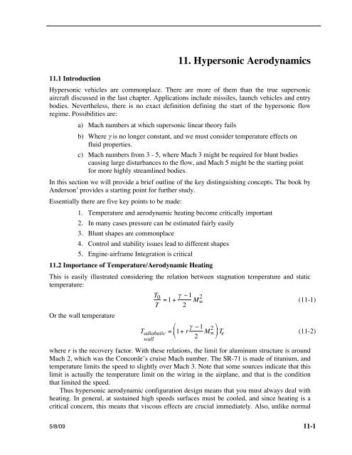
<strong>11.</strong>1 Introduction<br />
<strong>11.</strong> <strong>Hypersonic</strong> <strong>Aerodynamics</strong><br />
<strong>Hypersonic</strong> vehicles are commonplace. There are more of <strong>the</strong>m than <strong>the</strong> true supersonic<br />
aircraft discussed in <strong>the</strong> last chapter. Applications include missiles, launch vehicles and entry<br />
bodies. Never<strong>the</strong>less, <strong>the</strong>re is no exact definition defining <strong>the</strong> start of <strong>the</strong> hypersonic flow<br />
regime. Possibilities are:<br />
a) Mach numbers at which supersonic linear <strong>the</strong>ory fails<br />
b) Where γ is no longer constant, and we must consider temperature effects on<br />
fluid properties.<br />
c) Mach numbers from 3 - 5, where Mach 3 might be required for blunt bodies<br />
causing large disturbances to <strong>the</strong> flow, and Mach 5 might be <strong>the</strong> starting point<br />
for more highly streamlined bodies.<br />
In this section we will provide a brief outline of <strong>the</strong> key distinguishing concepts. The book by<br />
Anderson 1 provides a starting point for fur<strong>the</strong>r study.<br />
Essentially <strong>the</strong>re are five key points to be made:<br />
1. Temperature and aerodynamic heating become critically important<br />
2. In many cases pressure can be estimated fairly easily<br />
3. Blunt shapes are commonplace<br />
4. Control and stability issues lead to different shapes<br />
5. Engine-airframe Integration is critical<br />
<strong>11.</strong>2 Importance of Temperature/Aerodynamic Heating<br />
This is easily illustrated considering <strong>the</strong> relation between stagnation temperature and static<br />
temperature:<br />
Or <strong>the</strong> wall temperature<br />
T 0<br />
T<br />
T adiabatic<br />
wall<br />
γ −1 2<br />
=1 + M<br />
2 ∞<br />
⎛<br />
= ⎜ 1+ r γ −1<br />
2 M ∞ 2<br />
⎝<br />
(11-1)<br />
⎞<br />
⎟ T<br />
⎠ e (11-2)<br />
where r is <strong>the</strong> recovery factor. With <strong>the</strong>se relations, <strong>the</strong> limit for aluminum structure is around<br />
Mach 2, which was <strong>the</strong> Concorde’s cruise Mach number. The SR-71 is made of titanium, and<br />
temperature limits <strong>the</strong> speed to slightly over Mach 3. Note that some sources indicate that this<br />
limit is actually <strong>the</strong> temperature limit on <strong>the</strong> wiring in <strong>the</strong> airplane, and that is <strong>the</strong> condition<br />
that limited <strong>the</strong> speed.<br />
Thus hypersonic aerodynamic configuration design means that you must always deal with<br />
heating. In general, at sustained high speeds surfaces must be cooled, and since heating is a<br />
critical concern, this means that viscous effects are crucial immediately. Also, unlike normal<br />
5/8/09 11-1
11-2 Configuration <strong>Aerodynamics</strong><br />
airplane aerodynamics, hypersonic vehicles fly at very high altitudes, and <strong>the</strong> Reynolds<br />
number may be so low that <strong>the</strong> flow is laminar. Thus laminar flows are often of interest. This<br />
is important because <strong>the</strong> heat transfer is much lower when <strong>the</strong> flow is laminar. In fact, being<br />
able to estimate <strong>the</strong> transition location with certainty is a critical requirement in hypersonic<br />
vehicle design, and is <strong>the</strong> subject of current research. 2<br />
The X-15, shown in Figure 11-1, is <strong>the</strong> only real manned hypersonic airplane flown to<br />
date. It was rocket powered, and started flight by being dropped from a B-52, so it was purely<br />
a research airplane. The first flight was by Scott Crossfield in June of 1959. The X-15 reached<br />
314,750 feet in July of 1962. An improved version reached a Mach number of 6.7 and an<br />
altitude of 102,100 feet in October of 1967 with Pete Knight at <strong>the</strong> controls. The X-15<br />
program flew 199 flights, with <strong>the</strong> last one being in October of 1968. * Milt Thompson’s book 3<br />
describes <strong>the</strong> X-15 program, including <strong>the</strong> crackling sounds in <strong>the</strong> airframe as it heated up!<br />
Figure 11-1. X-15 (NASA Dryden photo archives photo)<br />
In case <strong>the</strong> issue of aerodynamic heating seems academic, consider <strong>the</strong> M = 6.7 flight of<br />
<strong>the</strong> X-15. It turned out to be <strong>the</strong> last flight of that plane. A dummy ramjet installation was<br />
* The only undergraduate from <strong>the</strong> <strong>Virginia</strong> <strong>Tech</strong> Aerospace Engineering program to earn astronaut status was<br />
Jack McKay, who flew <strong>the</strong> X-15 as a NASA test pilot, and reached 295,000 feet in September of 1965.<br />
5/8/09
W.H. Mason <strong>Hypersonic</strong> <strong>Aerodynamics</strong> 11-3<br />
tested by placing <strong>the</strong> ramjet mockup below <strong>the</strong> airplane. The shocks from <strong>the</strong> front of <strong>the</strong><br />
ramjet inlet spike impinged on <strong>the</strong> pylon supporting <strong>the</strong> scramjet. The shock interference<br />
heating was so severe that <strong>the</strong> shocks acted as a blowtorch, cutting through <strong>the</strong> structure, and<br />
effectively slicing off <strong>the</strong> scramjet. The internal damage to <strong>the</strong> airplane from <strong>the</strong> heating led to<br />
<strong>the</strong> scrapping of this high-speed version of <strong>the</strong> airplane. Figure 11-2 below shows <strong>the</strong> scramjet<br />
hanging below <strong>the</strong> airplane.<br />
Figure 11-2. X-15 with dummy ramjet (Picture from <strong>the</strong> NASA Dryden Photo Web Site)<br />
<strong>11.</strong>3 Surface pressure estimation<br />
In many cases surface pressures are relatively easy to estimate at hypersonic speeds. At<br />
supersonic speed we have a local relation for two-dimensional flows relating surface slope<br />
and pressure:<br />
C p =<br />
2θ<br />
M 2 −1<br />
(11-3)<br />
However, this relation is not particularly useful in most cases on actual aircraft<br />
configurations. In comparison, hypersonic rules are useful. The most famous relation is based<br />
on <strong>the</strong> concepts of Newton. Although Newton was wrong for low-speed flow, his idea does<br />
apply at hypersonic speeds. The idea is that <strong>the</strong> oncoming flow can be though of as a stream<br />
of particles, which lose all <strong>the</strong>ir momentum normal to a surface when <strong>the</strong>y “hit” <strong>the</strong> surface.<br />
This leads to <strong>the</strong> relation:<br />
C p = 2sin 2 θ (11-4)<br />
where θ is <strong>the</strong> angle between <strong>the</strong> flow vector and <strong>the</strong> surface. Thus you only need to know <strong>the</strong><br />
geometry of <strong>the</strong> body locally to estimate <strong>the</strong> local surface pressure. Also, particles impact only<br />
<strong>the</strong> portion of <strong>the</strong> body facing <strong>the</strong> flow, as shown in Figure 11-3. The rest of <strong>the</strong> body is in a<br />
“shadow”, and <strong>the</strong> Cp is zero. See Anderson 1 for <strong>the</strong> derivation of this and o<strong>the</strong>r pressureslope<br />
rules.<br />
Two key observations come from <strong>the</strong> Newtonian rule. First, <strong>the</strong> Mach number does not<br />
appear! Second, <strong>the</strong> pressure is related to <strong>the</strong> square of <strong>the</strong> inclination angle and not linearly as<br />
it is in <strong>the</strong> supersonic formula. This illustrates how <strong>the</strong> situation in hypersonic flow is<br />
significantly different than <strong>the</strong> linearized flow models at lower speed.<br />
5/8/09
11-4 Configuration <strong>Aerodynamics</strong><br />
oncoming<br />
flow<br />
Shadow<br />
Region,<br />
Cp = 0.0<br />
Figure 11-3. Shadow sketch, showing region where Cp is zero<br />
This figure also shows how <strong>the</strong> situation changes from low speed to high speed. Look at <strong>the</strong><br />
“ultimate” lift plot in Figure 11-4. Here <strong>the</strong> lower surface pressure is taken equal to <strong>the</strong><br />
stagnation value, and <strong>the</strong> upper surface is taken equal to <strong>the</strong> vacuum value. We can see that at<br />
low speeds <strong>the</strong> lift is generated on <strong>the</strong> upper surface, while at high speed <strong>the</strong> lift is almost<br />
completely generated on <strong>the</strong> lower surface.<br />
CL<br />
ultimate<br />
14.0<br />
12.0<br />
10.0<br />
8.0<br />
"Ultimate" CL<br />
Note <strong>the</strong> switch from upper surface<br />
to lower surface dominated, and <strong>the</strong><br />
relatively low values from Mach 0.9<br />
to Mach 1.5.<br />
6.0<br />
Total Lift<br />
4.0<br />
Upper<br />
Surface<br />
2.0<br />
Lower<br />
Surface<br />
0.0<br />
0.0 0.5 1.0 1.5 2.0 2.5 3.0<br />
Mach<br />
Figure 11-4. The “Ultimate CL” plot (showing <strong>the</strong> dominance of <strong>the</strong> lower<br />
surface at hypersonic speeds)<br />
The Newtonian flow model can be refined to improve agreement with data. This form is<br />
known as <strong>the</strong> Modified Newtonian flow formula,<br />
where <strong>the</strong> stagnation Cp is a function of Mach and γ,<br />
C p = C pmax sin 2 θ (11-5)<br />
C pmax = p 0 2<br />
− p ∞<br />
1 2<br />
ρ ∞ V ∞<br />
2 (11-6)<br />
and P 02 is <strong>the</strong> stagnation or total pressure behind a normal shock. This expression gets both <strong>the</strong><br />
Mach number and ratio of specific heats back into <strong>the</strong> problem. The classical Newtonian<br />
5/8/09
W.H. Mason <strong>Hypersonic</strong> <strong>Aerodynamics</strong> 11-5<br />
<strong>the</strong>ory is actually <strong>the</strong> limit as M → ∞, and γ → 1. As briefly noted above, <strong>the</strong>re are lots of<br />
o<strong>the</strong>r local rules, and Anderson’s book 1 should be consulted for a complete discussion.<br />
<strong>11.</strong>4 Round LE shapes to reduce heat transfer<br />
Since round shapes have lots of drag, why do we see such highly rounded shapes The answer<br />
is <strong>the</strong> heat transfer. The maximum value of <strong>the</strong> heat transfer is related to <strong>the</strong> leading edge<br />
radius as shown in this relation:<br />
q ˙ max ≈<br />
laminar<br />
1<br />
R LE<br />
(11-7)<br />
where R LE is <strong>the</strong> leading edge radius at <strong>the</strong> stagnation point.<br />
Thus, we need a nose or leading edge radius large enough for <strong>the</strong> tip not to melt. H. Julian<br />
Allen and A.J. Eggers, Jr., at NASA Ames did <strong>the</strong> analysis that showed that blunt bodies were<br />
required to survive entry from orbit. 4 Thus, <strong>the</strong> solution of hypersonic flows about <strong>the</strong> nose of<br />
an entering body became an important analysis problem. In fact, this was <strong>the</strong> first great<br />
challenge problem for CFD (this was in <strong>the</strong> 1960s, and <strong>the</strong> computational solution of <strong>the</strong><br />
flowfield wasn’t called CFD until <strong>the</strong> early 1970s). It is known as “<strong>the</strong> Blunt Body problem”.<br />
It was particularly difficult because <strong>the</strong> flow is subsonic behind a normal, or nearly normal,<br />
shock wave. The flow <strong>the</strong>n accelerates quickly to supersonic/hypersonic speed. This is <strong>the</strong><br />
reverse problem of transonic flow, where <strong>the</strong> freestream is supersonic/hypersonic ra<strong>the</strong>r than<br />
subsonic. In particular, we want to know <strong>the</strong> shock standoff distance, <strong>the</strong> shock shape, and <strong>the</strong><br />
flow properties at <strong>the</strong> nose, where <strong>the</strong> aerodynamic heating is largest. The shape of <strong>the</strong> shock<br />
determines <strong>the</strong> distribution of flow properties such as entropy, which vary as <strong>the</strong> shock shape<br />
changes.<br />
The problem was solved by computing <strong>the</strong> unsteady flowfield, which is always<br />
ma<strong>the</strong>matically hyperbolic. If <strong>the</strong> solution is actually steady, <strong>the</strong> computation will converge to<br />
<strong>the</strong> steady state result, while overcoming <strong>the</strong> difficulty of <strong>the</strong> mixed elliptic-hyperbolic<br />
equation type that describes <strong>the</strong> steady state problem. The successful method invented to<br />
obtain a practical blunt body calculation method is generally attributed to Moretti. 5<br />
<strong>11.</strong>5. Aerodynamic control<br />
We described <strong>the</strong> benefits of blunt shapes above. Many hypersonic vehicles display ano<strong>the</strong>r<br />
unusual geometric feature. It turns out that thick bases are often used on hypersonic vehicles,<br />
and in this section we illustrate why <strong>the</strong>y are desirable. Our example relates to <strong>the</strong> thick<br />
trailing edge on <strong>the</strong> vertical tail of <strong>the</strong> X-15.<br />
The example of <strong>the</strong> difference in <strong>the</strong> flow characteristics between supersonic and<br />
hypersonic speed can be illustrated with <strong>the</strong> hypersonic directional stability problem. To start,<br />
we consider <strong>the</strong> yawing moment, which is<br />
where <strong>the</strong> standard definition of C N is:<br />
N VT = q VT S VT l VT C YVT (11-8)<br />
C n =<br />
N<br />
q ref S ref b ref<br />
(11-9)<br />
5/8/09
11-6 Configuration <strong>Aerodynamics</strong><br />
We can write <strong>the</strong> yawing moment due to <strong>the</strong> vertical tail as:<br />
C nVT =<br />
l VT S VT<br />
b ref S<br />
ref<br />
<br />
vertical tail<br />
volume<br />
coefficient, V VT<br />
q VT<br />
⋅ C YVT (11-10)<br />
q<br />
ref<br />
ratio of<br />
dynamic pressures<br />
assume ≈ 1<br />
The nomenclature associated with <strong>the</strong> problem and <strong>the</strong> equations is illustrated in Figure 11-5.<br />
⋅<br />
β<br />
V<br />
∞<br />
N<br />
l VT<br />
Y VT<br />
US<br />
LS<br />
θ<br />
Figure 11-5. Sketch defining <strong>the</strong> hypersonic directional stability problem<br />
Now, for a high-speed flow, we will assume that <strong>the</strong> vertical tail is a two-dimensional<br />
surface with a constant pressure on each side, so that C YVT = C PLS − C PUS . We will consider<br />
two cases, one supersonic, <strong>the</strong> o<strong>the</strong>r hypersonic. We compare <strong>the</strong> results for directional<br />
stability at high Mach number using <strong>the</strong> two-dimensional rule for linearized supersonic flow<br />
and Newtonian <strong>the</strong>ory for hypersonic flow, as shown below.<br />
θ<br />
5/8/09
W.H. Mason <strong>Hypersonic</strong> <strong>Aerodynamics</strong> 11-7<br />
Linear <strong>the</strong>ory<br />
2θ<br />
C p =<br />
M 2 −1<br />
Newtonian <strong>the</strong>ory<br />
C p = 2sin 2 θ (11-11)<br />
Case 1: Linearized supersonic <strong>the</strong>ory<br />
( )<br />
( )<br />
C YVT = ΔC p = 2 θ + β<br />
M 2 −1 − 2 θ − β<br />
M 2 −1 =<br />
showing that <strong>the</strong> θ’s cancel. We use this expression to get C nβ :<br />
C nβ<br />
VT = V VT<br />
∂C YVT<br />
∂β<br />
= V VT<br />
4<br />
M 2 −1<br />
4β<br />
M 2 −1<br />
This expression shows that C nβ is positive, but vanishes for hypersonic Mach numbers.<br />
(11-12)<br />
(11-13)<br />
Case 2: <strong>Hypersonic</strong> flow <strong>the</strong>ory, Newtonian <strong>the</strong>ory<br />
This time <strong>the</strong> expression for <strong>the</strong> side force is:<br />
Using trig functions:<br />
Which reduces to:<br />
and<br />
C Yβ<br />
VT<br />
C YVT = ΔC p = 2sin 2 ( θ + β) − 2sin 2 ( θ − β) (11-14)<br />
⎡<br />
= 2 sin2 θ cos 2 β + 2cosθ sinβ sinθ cos β + cos 2 θ sin 2 β<br />
⎤<br />
⎢<br />
⎥<br />
⎢<br />
⎣ −sin 2 θ cos 2 β + 2 cosθ sin βsinθ cos β − cos 2 θ sin 2 ⎥<br />
β⎦<br />
C YβVT<br />
= 8cosθ sin β<br />
sinθ cosβ <br />
≈1 ≈β ≈θ ≈1<br />
≅ 8θβ<br />
(11-15)<br />
(11-16)<br />
C nβ<br />
VT = 8V VTθ (11-17)<br />
If θ is zero, so is C nβ ! But opening up <strong>the</strong> wedge angle rapidly increases C nβ . In addition,<br />
<strong>the</strong>re is no Mach number dependence. The Case 2 results were verified experimentally, and<br />
<strong>the</strong> wedge vertical tail concept literally saved <strong>the</strong> X-15 program. 6 This effect is also <strong>the</strong> reason<br />
for flared “skirts” seen on some launch vehicles.<br />
The application of this effect is clearly shown in <strong>the</strong> first picture of <strong>the</strong> X-15 above and <strong>the</strong><br />
front view of <strong>the</strong> X-15 shown in Figure 11-6 below.<br />
5/8/09
11-8 Configuration <strong>Aerodynamics</strong><br />
Figure 11-6. Picture of <strong>the</strong> X-15 showing <strong>the</strong> wedge used for <strong>the</strong> vertical tail “airfoil”<br />
section. (from <strong>the</strong> US Air Force Museum Web Site)<br />
<strong>11.</strong>6. Engine-airframe Integration<br />
Any air-breathing hypersonic vehicle will have a highly integrated engine and airframe. It will<br />
be hard to tell exactly what counts as <strong>the</strong> vehicle, and what counts as <strong>the</strong> propulsion system.<br />
This is exemplified in <strong>the</strong> concepts developed for recent aerospace planes. In <strong>the</strong>se concepts<br />
<strong>the</strong> propulsion is at least in part provided by a scramjet engine, which obtains thrust with a<br />
combustion chamber in which <strong>the</strong> flow is supersonic. Figure 11-7, from a presentation by<br />
Walt Engelund of NASA Langley, shows this concept. The entire forebody of <strong>the</strong> vehicle<br />
underside is used as an external inlet to provide flow at just <strong>the</strong> right conditions to <strong>the</strong> engine.<br />
The entire underside afterbody is <strong>the</strong> exhaust nozzle.<br />
The first US vehicle to use a scramjet engine was <strong>the</strong> Hyper-X, now known as <strong>the</strong> X-43.<br />
The initial flight attempt was made in June of 2001, but failed before having a chance to<br />
demonstrate <strong>the</strong> operation of <strong>the</strong> scramjet. After a long investigation and a revised procedure,<br />
it flew successfully on March 27, 2004. 7 The X-43A is shown in <strong>the</strong> Figures 11-8 and 11-9.<br />
The November-December 2001 issue of <strong>the</strong> Journal of Spacecraft and Rockets had a<br />
special section devoted to <strong>the</strong> Hyper-X.<br />
5/8/09
W.H. Mason <strong>Hypersonic</strong> <strong>Aerodynamics</strong> 11-9<br />
Figure 11-7. Example of engine-airframe integration for a hypersonic aircraft<br />
(from Walt Engelund, NASA Langley, May 2001).<br />
Figure 11-8. Artist conception of <strong>the</strong> X-43<br />
5/8/09
11-10 Configuration <strong>Aerodynamics</strong><br />
Figure 11-9. The X-43 at NASA Dryden in flight preparation early in 2001.<br />
<strong>11.</strong>7 Airbreathing <strong>Hypersonic</strong> Vehicle Design<br />
The successful design of an airbreathing hypersonic vehicle is an excellent example of <strong>the</strong><br />
need for multidisciplinary optimization methods. This is a very hard problem. The recent<br />
success of <strong>the</strong> scramjet test flight means that we can expect to see designs proposed using this<br />
technology. Key surveys are available based on numerous studies conducted at NASA<br />
Langley. 8,9<br />
Finally, we note that one concept not discussed so far deserves mention. Waveriders<br />
potentially provide efficient hypersonic flight. These designs can be thought of as placing a<br />
shape in <strong>the</strong> streamline of body generated flowfield so that <strong>the</strong> bottom surface is resting on <strong>the</strong><br />
pressure field generated by <strong>the</strong> shock wave of this flowfield. The arrangement is designed to<br />
obtain lift with very low drag. 10<br />
<strong>11.</strong>10 Exercises<br />
1. Derive expressions for <strong>the</strong> lift curve slope of a flat plate and a wedge using linearized<br />
supersonic <strong>the</strong>ory and Newtonian <strong>the</strong>ory. Comment on <strong>the</strong> differences.<br />
<strong>11.</strong>9 References<br />
1 John Anderson, <strong>Hypersonic</strong> and High Temperature Gas Dynamics, McGraw-Hill, New<br />
York, 1989. (reissued as a second edition by <strong>the</strong> AIAA)<br />
2 John J. Bertin and Russell M. Cummings, “Fifty years of hypersonics: where we’ve been,<br />
where we’re going”, Progress in Aerospace Sciences, Vol. 39, pp. 511-536, 2003 (Note:<br />
ignore <strong>the</strong> error in <strong>the</strong> first line of <strong>the</strong> abstract, that has <strong>the</strong> wrong date and pilot for <strong>the</strong> Mach<br />
6.7 flight)<br />
5/8/09
W.H. Mason <strong>Hypersonic</strong> <strong>Aerodynamics</strong> 11-11<br />
3 Milton O. Thompson, At <strong>the</strong> Edge of Space: The X-15 Flight Program, Smithsonian<br />
Institution Press, Washington, 1992.<br />
4 H. Julian Allen and A.J. Eggers, Jr., “A Study of <strong>the</strong> Motion and Aerodynamic Heating of<br />
Ballistic Missiles Entering <strong>the</strong> Earth’s Atmosphere at High Supersonic Speeds,” NACA<br />
Report 1381, 1958.<br />
5 Gino Moretti and Mike Abbett, “A Time Dependent Computational Method for Blunt Body<br />
Flows,” AIAA Journal, Vol. 4, No. 12, 1966, pp. 2136-2141.<br />
6 Charles McLellan, “A Method for Increasing <strong>the</strong> Effectiveness of Stabilizing Surfaces at<br />
High Supersonic Mach Numbers,” NACA RM L54F21, Aug. 1954, Declassified: 1958.<br />
7 Michael A. Dornheim, “A Breath of Fast Air,” Aviation Week & Space <strong>Tech</strong>nology, April 5,<br />
2004.<br />
8 Mary K. O’Neill and Mark J. Lewis, “Design Tradeoffs on Engine-Integrated <strong>Hypersonic</strong><br />
Vehicles,” AIAA Paper 92-1205, Feb. 1992.<br />
9<br />
Mary K. Lockwood, Dennis H. Petley, John G. Martin and James L. Hunt, “Airbreathing<br />
hypersonic vehicle design and analysis methods and interactions,” Progress in Aerospace<br />
Sciences, Vol. 35, pp. 1-32, 1999.<br />
10 Charles E. Cockrell, Jr., Lawrence D. Huebner and Dennis B. Finley, “Aerodynamic<br />
Characteristics of Two Waverider-Derived <strong>Hypersonic</strong> Cruise Configurations,” NASA TP<br />
3559, July 1996.<br />
5/8/09