marees terrestres bulletin d'informations - UniversitÃ© de la PolynÃ©sie ...

More documents

Recommendations

Info

Planets Space, 59, 307–311. Sato, T., Tamura, Y., Matsumoto, K., Imanishi, Y. and McQueen, H., 2004. Parameters of the fluid core resonance inferred from superconducting gravimeter data, J. Geodyn., 38, 375-389. Sato, Tadahiro, Jun’ichi Okuno, Jacques Hinderer, Daniel S. MacMillan, Hans-Peter Plag, Olivier Francis, Reinhard Falk, and Yoichi Fukuda, 2006. A geophysical interpretation of the secular displacement and gravity rates observed at Ny-Ålesund, Svalbard in the Arctic - Effects of post-glacial rebound and present-day ice melting -, G. J. Int., 165., 729-743, doi: 10.IIII/j.1365-246x.2006.02992.x. T. Sato, S. Miura, Y. Ohta, H. Fujimoto, W. Sun, C.F. Larsen, M. Heavner, A.M. Kaufman, J.T. Freymueller, 2008. Earth tides observed by gravity and GPS in southeastern Alaska, J. Geodyn., 46, 78–89. Schenewerk, M. S., J. Marshall and W. Dillingar (2001), Vertical Ocean-loading Deformations Derived from a Global GPS Network, J. Geod. Soc. Japan, Vol.47, No.1, 237-242. Schwiderski, E. W. (1980), On charting global ocean tides, Rev. Geophys. Space Phys., 18, 243-268. Takasu, T., and Kasai, S., 2005. Development of precise orbit/clock determination software for GPS/GNSS, Proce. the 49th Space Sciences and Technology Conference, Hiroshima, Japan (in Japanese), 1223-1227. Takasu, T., 2006. High-rate Precise Point Positioning: Detection of crustal deformation by using 1-Hz GPS data, GPS/GNSS symposium 2006, Tokyo, 52-59. Tamura Y., Sato, T., Ooe, M. and Ishiguro, M., 1991. A procedure for tidal analysis with a Bayesian information criterion, Geophys. J. Int., 104, 507-516. Thomas, I. D., King, M. A., Clarke, P. J., 2007. A comparison of GPS, VLBI and model estimates of ocean tide loading displacements, J. Geodesy, 81(5), 359-268. Wahr, J. M., 1981. Body tides of an elliptical, rotating, elastic and oceanless Earth, Geophys. R. Astron. Soc., 64, 677-703. Wang, R., 1991. Tidal deformations of a rotating, spherically symmetric, visco-elastic and laterally heterogeneous Earth, Ph.D. Thesis, Univ. of Kiel, Kiel, Germany. Widmer-Schnidrig, R., 2003. What can superconducting gravimeters contribute to normal mode seismology, Bull. Seism. Soc. Am., 93(3), 1370–1380. Zumberge, J. F., Heflin, M. B., Jefferson, D. C., Watkins, M. M., and Webb, F. H., 1997. Precise point positioning for the efficient and robust analysis of GPS data from large networks, J. Geophys. Res., 102 (B3), 5005-5017. Zürn, W., Beaumont, C. and Slichter, L. B., 1976. Gravity tides and ocean loading in southern Alaska, J. Geophys. Res., Vol. 81, No. 26, 4923-4932. 11762
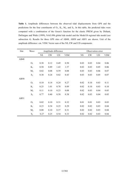
Table 1. Amplitude differences between the observed tidal displacements from GPS and the predictions for the four constituents of O 1 , K 1 , M 2 , and S 2 . In this table, the predicted tides were computed with a combination of the Green’s function for the elastic PREM given by Dehant, Defraigne and Wahr (1999), NAO.99b global tide model and the Model B regional tide model (see subsection 4). Results for three GPS sites of AB48, AB50 and AB51 are shown. Unit of the amplitude difference: cm. VSM: Vector sum of the NS, EW and UD components. Site Wave Amplitude difference Observation error NS EW UD VSM NS EW UD VSM AB48 O 1 0.38 0.12 0.49 0.50 0.03 0.03 0.04 0.06 K 1 0.50 0.89 1.43 1.57 0.03 0.03 0.05 0.06 M 2 0.02 0.08 0.59 0.08 0.03 0.03 0.06 0.07 S 2 0.38 0.24 0.82 0.43 0.03 0.03 0.05 0.07 AB50 O 1 0.10 0.14 0.24 0.27 0.02 0.10 0.03 0.11 K 1 0.25 1.01 0.78 0.89 0.02 0.10 0.03 0.10 M 2 0.11 0.10 0.23 0.08 0.02 0.03 0.04 0.05 S 2 0.77 0.40 0.58 0.38 0.02 0.03 0.04 0.05 AB51 O 1 0.02 0.10 0.31 0.32 0.01 0.01 0.03 0.03 K 1 0.23 0.34 0.25 0.29 0.02 0.02 0.03 0.04 M 2 0.08 0.10 0.37 0.31 0.02 0.02 0.03 0.04 S 2 0.27 0.25 0.54 0.33 0.02 0.02 0.03 0.04 11763
Page 1: MAREES TERRESTRES BULLETIN D'INFORM
Page 6 and 7: BIM 146 December 15, 2010 New Chall
Page 8 and 9: 1994), and TPXO.6 (Egbert et al., 1
Page 10 and 11: 4. An attempt to improve the region
Page 12 and 13: From Fig. 2, we also see that, the
Page 14 and 15: GPS network called GEONET (GPS Eart
Page 16 and 17: References Bos, M. S., Baker, T. F.
Page 20 and 21: Fig. 1. Locations of the observatio
Page 22 and 23: BLANK PAGE
Page 24 and 25: the dense seismic observation netwo
Page 26 and 27: difference of loading effects of oc
Page 28 and 29: is done with an optical lever using
Page 30 and 31: 6. Application of laser interferome
Page 32 and 33: Figure 11. Strain seismograms of th
Page 34 and 35: Higashi, T., 1996, A study on chara
Page 38 and 39: 2. Fundamentals and techniques At t
Page 40 and 41: 100 low frequencies earth tide freq
Page 42 and 43: Tab. 4: Averages of noise levels at
Page 44 and 45: References Asch, G., Elstner, C., J
Page 46 and 47: The 1 / s part is also worth mentio
Page 48 and 49: As it was mentioned before the resu
Page 50 and 51: Fig. 9. Morlet Wavelet Spectrum, su
Page 52 and 53: 9. CONCLUSIONS This investigation w
Page 54 and 55: 2. Objectives of Aswan Tidal Gravit
Page 56 and 57: 5. Recording of Data The data logge
Page 58 and 59: Figure 5: Pre-processed hourly data
Page 60 and 61: Figure 6: Residuals of gravity tide
Page 64 and 65: time. In addition, models for gravi
Page 66 and 67: Fig. 3 (Zahran, 2005) shows gravity
Page 68 and 69:
during the years 2003 and 2004. It
Page 70 and 71:
Figure 7: Variation of phase shift,
Page 72 and 73:
Figure 8: Induced gravity load and
Page 74 and 75:
BLANK PAGE
Page 76 and 77:
The instrumentation of the tidal st
Page 78 and 79:
4. Tidal analysis The tidal analysi
Page 80 and 81:
References Banka, D., Crossley, D.
Page 82 and 83:
1. Introduction The estimation of a
Page 84 and 85:
Figure 1 Air density distributions
Page 86 and 87:
temperature effect is considered, t
Page 88 and 89:
Figure 4 Attraction effect from the
Page 90 and 91:
a ) up to 0.5° , b) 0.5°- 1.5° ,
Page 92 and 93:
Figure 7 Atmospheric reductions for
Page 94 and 95:
Figure 9 Amplitude spectra of diffe
Page 96 and 97:
Figure 10 SG observation and gravit
Page 98 and 99:
eduction in the long-period tides r
Page 100 and 101:
oceans. The effect has a peak-to-pe
Page 102 and 103:
BLANK PAGE
Page 104 and 105:
Figure 1. Local earthquakes recorde
Page 106 and 107:
4. Recording of Data The recorded d
Page 108 and 109:
Table 1: Adjusted tidal parameters
Page 110 and 111:
Acknowledgements: The authors are i
Page 112:
BLANK PAGE
show all

marees terrestres bulletin d'informations - UniversitÃ© de la PolynÃ©sie ...

Create successful ePaper yourself

Delete template?

Save as template?