marees terrestres bulletin d'informations - UniversitÃ© de la PolynÃ©sie ...

More documents

Recommendations

Info

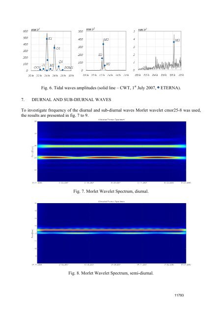
As it was mentioned before the results of the CWT is the matrix of C-coefficients, which are the amounts of the energy in particular periods. To recalculate it into amplitude the linear relationship was used (Kalarus, 2007): where: A A is the amplitude, C - wavelet coefficient, C n - integral from the envelope of the wavelet function used for calculations. C n ⋅C (6) = 1 days In practice, C n is calculated by making wavelet transform of the artificial signal of amplitude 1 and period determined by the transform of the original signal. The C n coefficients obtained by this method are different for different frequencies (Fig. 5). 6. COMPARISON Fig. 5. Calculated values of C n factors. The amplitudes obtained by this method were compared to those determined using classical least square manner (Chojnicki, 1977) calculated using Eterna 3.4 (Wenzel, 1996) with the same original signal of gravity changes (see table 1). Table 1. Frequencies of the tidal waves. Frequency [cycle/day] Amplitude Std. dev. Name from to [nm/s^2] [nm/s^2] 0.501370 0.842147 SGQ1 2,76 0,143 0.842148 0.860293 2Q1 8,83 0,135 0.860294 0.878674 SGM1 10,45 0,137 0.878675 0.896968 Q1 66,09 0,127 0.896969 0.911390 RO1 12,53 0,131 0.911391 0.931206 O1 346,55 0,124 0.931207 0.949286 TAU1 4,61 0,165 0.949287 0.967660 M1 27,19 0,109 0.967661 0.981854 CHI1 5,37 0,122 0.981855 0.996055 PI1 9,15 0,149 0.996056 0.998631 P1 161,06 0,156 0.998632 1.001369 S1 3,49 0,227 1.001370 1.004107 K1 480,85 0,140 1.004108 1.006845 PSI1 4,49 0,150 1.006846 1.023622 PHI1 7,07 0,156 1.023623 1.035250 TET1 5,21 0,132 Frequency [cycle/day] Amplitude Std. dev. Name from to [nm/s^2] [nm/s^2] 1.035251 1.054820 J1 27,45 0,124 1.054821 1.071833 SO1 4,61 0,128 1.071834 1.090052 OO1 14,85 0,089 1.090053 1.470243 NU1 2,85 0,087 1.470244 1.845944 EPS2 2,43 0,058 1.845945 1.863026 2N2 8,44 0,061 1.863027 1.880264 MU2 10,21 0,067 1.880265 1.897351 N2 64,11 0,065 1.897352 1.915114 NU2 12,23 0,068 1.915115 1.950493 M2 335,38 0,068 1.950493 1.970390 L2 9,60 0,102 1.970391 1.998996 T2 9,15 0,065 1.998997 2.001678 S2 155,54 0,066 2.001679 2.468043 K2 42,40 0,049 2.468044 7.000000 M3M6 3,64 0,037 From the comparison we can notice that there is a big discrepancy in K1 frequency. We can claim that classical manner based on the least squares method better separate P1, K1 and S1 waves. The same conclusion could be pointed out: wavelet transform of this signal did not separated correctly S2 and K2 waves (see fig. 6).
Fig. 6. Tidal waves amplitudes (solid line – CWT, 1 st July 2007, ETERNA). 7. DIURNAL AND SUB-DIURNAL WAVES To investigate frequency of the diurnal and sub-diurnal waves Morlet wavelet cmor25-8 was used, the results are presented in fig. 7 to 9. Fig. 7. Morlet Wavelet Spectrum, diurnal. Fig. 8. Morlet Wavelet Spectrum, semi-diurnal.
Page 1: MAREES TERRESTRES BULLETIN D'INFORM
Page 6 and 7: BIM 146 December 15, 2010 New Chall
Page 8 and 9: 1994), and TPXO.6 (Egbert et al., 1
Page 10 and 11: 4. An attempt to improve the region
Page 12 and 13: From Fig. 2, we also see that, the
Page 14 and 15: GPS network called GEONET (GPS Eart
Page 16 and 17: References Bos, M. S., Baker, T. F.
Page 18 and 19: Planets Space, 59, 307-311. Sato, T
Page 20 and 21: Fig. 1. Locations of the observatio
Page 22 and 23: BLANK PAGE
Page 24 and 25: the dense seismic observation netwo
Page 26 and 27: difference of loading effects of oc
Page 28 and 29: is done with an optical lever using
Page 30 and 31: 6. Application of laser interferome
Page 32 and 33: Figure 11. Strain seismograms of th
Page 34 and 35: Higashi, T., 1996, A study on chara
Page 38 and 39: 2. Fundamentals and techniques At t
Page 40 and 41: 100 low frequencies earth tide freq
Page 42 and 43: Tab. 4: Averages of noise levels at
Page 44 and 45: References Asch, G., Elstner, C., J
Page 46 and 47: The 1 / s part is also worth mentio
Page 50 and 51: Fig. 9. Morlet Wavelet Spectrum, su
Page 52 and 53: 9. CONCLUSIONS This investigation w
Page 54 and 55: 2. Objectives of Aswan Tidal Gravit
Page 56 and 57: 5. Recording of Data The data logge
Page 58 and 59: Figure 5: Pre-processed hourly data
Page 60 and 61: Figure 6: Residuals of gravity tide
Page 64 and 65: time. In addition, models for gravi
Page 66 and 67: Fig. 3 (Zahran, 2005) shows gravity
Page 68 and 69: during the years 2003 and 2004. It
Page 70 and 71: Figure 7: Variation of phase shift,
Page 72 and 73: Figure 8: Induced gravity load and
Page 76 and 77: The instrumentation of the tidal st
Page 78 and 79: 4. Tidal analysis The tidal analysi
Page 80 and 81: References Banka, D., Crossley, D.
Page 82 and 83: 1. Introduction The estimation of a
Page 84 and 85: Figure 1 Air density distributions
Page 86 and 87: temperature effect is considered, t
Page 88 and 89: Figure 4 Attraction effect from the
Page 90 and 91: a ) up to 0.5° , b) 0.5°- 1.5° ,
Page 92 and 93: Figure 7 Atmospheric reductions for
Page 94 and 95: Figure 9 Amplitude spectra of diffe
Page 96 and 97: Figure 10 SG observation and gravit
Page 98 and 99:
eduction in the long-period tides r
Page 100 and 101:
oceans. The effect has a peak-to-pe
Page 102 and 103:
BLANK PAGE
Page 104 and 105:
Figure 1. Local earthquakes recorde
Page 106 and 107:
4. Recording of Data The recorded d
Page 108 and 109:
Table 1: Adjusted tidal parameters
Page 110 and 111:
Acknowledgements: The authors are i
Page 112:
BLANK PAGE
show all

marees terrestres bulletin d'informations - UniversitÃ© de la PolynÃ©sie ...

Create successful ePaper yourself

Delete template?

Save as template?