State estimation with Kalman Filter
State estimation with Kalman Filter
State estimation with Kalman Filter

Create successful ePaper yourself
Turn your PDF publications into a flip-book with our unique Google optimized e-Paper software.
Chapter 8<br />
<strong>State</strong> <strong>estimation</strong> <strong>with</strong><br />
<strong>Kalman</strong> <strong>Filter</strong><br />
8.1 Introduction<br />
This chapter describes how to estimate the values of state variables of a<br />
dynamic system. Why can such state estimators be useful<br />
• Supervision: <strong>State</strong> estimates can provide valuable information<br />
about important variables in a physical process, for example feed<br />
composition to a reactor, flow variations to a separator, etc.<br />
• Control: In general, the more information the controller has about<br />
the process it controls, the better (mor accurate) it can control it.<br />
<strong>State</strong> estimators can be a practical or economical alternative to real<br />
measurements. For example, the environmental forces acting on a<br />
vessel can be used by the controller to better control the position of<br />
the vessel, as in Dynamic Positioning systems.<br />
Because the state estimators are kind of sensors implemented in software<br />
(computer programs) they are some times denoted soft sensors.<br />
This chapter describes the <strong>Kalman</strong> <strong>Filter</strong> which is the most important<br />
algorithm for state <strong>estimation</strong>. The <strong>Kalman</strong> <strong>Filter</strong> was developed by<br />
Rudolf E. <strong>Kalman</strong> around 1960 [7]. There is a continuous-time version of<br />
the <strong>Kalman</strong> <strong>Filter</strong> and several discrete-time versions. (The discrete-time<br />
versions are immediately ready for implementation in a computer<br />
program.) Here the predictor-corrector version of the discrete-time <strong>Kalman</strong><br />
101
F. Haugen: Kompendium for Kyb. 2 ved Høgskolen i Oslo 102<br />
<strong>Filter</strong> will be described. This version seems to be the most commonly used<br />
version.<br />
8.2 Observability<br />
A necessary condition for the <strong>Kalman</strong> <strong>Filter</strong> to work correctly is that the<br />
system for which the states are to be estimated, is observable. Therefore,<br />
you should check for observability before applying the <strong>Kalman</strong> <strong>Filter</strong>.<br />
(There may still be other problems that prevent the <strong>Kalman</strong> <strong>Filter</strong> from<br />
producing accurate state estimates, as a faulty or inaccurate mathematical<br />
model.)<br />
Observability for the discrete-time systems can be defined as follows [13]:<br />
The discrete-time system<br />
x(k +1)=Ax(k)+Bu(k) (8.1)<br />
y(k) =Cx(k)+Du(k) (8.2)<br />
is observable if there is a finite number of time steps k so that knowledge<br />
about the input sequence u(0),...,u(k − 1) and the output sequence<br />
y(0),...,y(k − 1) is sufficient to determine the initial state state of the<br />
system, x(0).<br />
Let us derive a criterion for the system to be observable. Since the<br />
influende of input u on state x is known from the model, let us for<br />
simplicity assume that u(k) =0. From the model (8.1) — (8.2) we get<br />
y(0) = Cx(0) (8.3)<br />
y(1) = Cx(1) = CAx(0) (8.4)<br />
.<br />
y(n − 1) = CA n−1 x(0) (8.5)<br />
whichcanbeexpressedcompactlyas<br />
⎡ ⎤ ⎡<br />
C<br />
CA<br />
⎢ ⎥x(0) = ⎢<br />
⎣ . ⎦ ⎣<br />
CA n−1<br />
| {z }<br />
M obs<br />
y(0)<br />
y(1)<br />
⎤<br />
⎥<br />
⎦<br />
.<br />
|<br />
y(n − 1)<br />
{z }<br />
Y<br />
(8.6)
F. Haugen: Kompendium for Kyb. 2 ved Høgskolen i Oslo 103<br />
Let us make a definition:<br />
Observability matrix:<br />
⎡ ⎤<br />
C<br />
CA<br />
M obs = ⎢ ⎥<br />
⎣ . ⎦<br />
CA n−1<br />
(8.7)<br />
(8.6) has a unique solution only if the rank of M obs is n. Therefore:<br />
Observability Criterion:<br />
The system (8.1) — (8.2) is observable if and only if the observability<br />
matrix has rank equal to n where n is the order of the system model (the<br />
number state variables).<br />
The rank can be checked by calculating the determinant of M obs .Ifthe<br />
determinant is non-zero, the rank is full, and hence, the system is<br />
observable. If the determinant is zero, system is non-observable.<br />
Non-observability has several concequences:<br />
• The transfer function from the input variable y to the output variable<br />
y has an order that is less than the number of state variables (n).<br />
• There are state variables or linear combinations of state variables<br />
that do not show any response.<br />
• The steady-state value of the <strong>Kalman</strong> <strong>Filter</strong> gain can not be<br />
computed. This gain is used to update the state estimates from<br />
measurements of the (real) system.<br />
Example 18 Observability<br />
Given the following state space model:<br />
· ¸ · ¸<br />
x1 (k +1) 1 a<br />
=<br />
x 2 (k +1) 0 1<br />
| {z }<br />
A<br />
·<br />
x1 (k)<br />
x 2 (k)<br />
y(k) = £ c 1 0 ¤ ·<br />
x1 (k)<br />
| {z } x 2 (k)<br />
C<br />
¸<br />
¸<br />
+ [0]<br />
· 0<br />
+<br />
1<br />
|{z}<br />
D<br />
| {z }<br />
B<br />
¸<br />
u(k) (8.8)<br />
u(k) (8.9)
F. Haugen: Kompendium for Kyb. 2 ved Høgskolen i Oslo 104<br />
The observability matrix is (n =2)<br />
⎡ £<br />
·<br />
¸<br />
c1 0 ¤ ⎤<br />
· ¸<br />
C<br />
M obs =<br />
CA 2−1 = ⎢ −−−−−−−−−−−<br />
= CA ⎣ £<br />
c1 0 ¤ · ¸ ⎥<br />
1 a ⎦ = c1 0<br />
c 1 ac 1<br />
0 1<br />
(8.10)<br />
The determinant of M obs is<br />
det (M obs )=c 1 · ac 1 − c 1 · 0=ac 1<br />
2<br />
(8.11)<br />
The system is observable only if ac 1 2 6=0.<br />
• Assume that a 6= 0which means that the first state variable, x 1 ,<br />
contains some non-zero information about the second state variable,<br />
x 2 . Then the system is observable if c 1 6=0,i.e.ifx 1 is measured.<br />
• Assume that a =0which means that x 1 contains no information<br />
about x 2 . In this case the system is non-observable despite that x 1 is<br />
measured.<br />
[End of Example 18]<br />
8.3 The <strong>Kalman</strong> <strong>Filter</strong> algorithm<br />
The <strong>Kalman</strong> <strong>Filter</strong> is a state estimator which produces an optimal<br />
estimate in the sense that the mean value of the sum (actually of any<br />
linear combination) of the <strong>estimation</strong> errors gets a minimal value. In other<br />
words, The <strong>Kalman</strong> <strong>Filter</strong> gives the following sum of squared errors:<br />
a minimal value. Here,<br />
E[e x T (k)e x (k)] = E £ e x1 2 (k)+···+ e xn 2 (k) ¤ (8.12)<br />
e x (k) =x est (x) − x(k) (8.13)<br />
is the <strong>estimation</strong> error vector. (The Kaman <strong>Filter</strong> estimate is sometimes<br />
denoted the “least mean-square estimate”.) This assumes actually that the<br />
model is linear, so it is not fully correct for nonlinear models. It is assumed<br />
the that the system for which the states are to be estimated is excited by<br />
random (“white”) disturbances ( or process noise) and that the
F. Haugen: Kompendium for Kyb. 2 ved Høgskolen i Oslo 105<br />
measurements (there must be at least one real measurement in a <strong>Kalman</strong><br />
<strong>Filter</strong>) contain random (“white”) measurement noise.<br />
The <strong>Kalman</strong> <strong>Filter</strong> has many applications, e.g. in dynamic positioning of<br />
ships where the <strong>Kalman</strong> <strong>Filter</strong> estimates the position and the speed of the<br />
vessel and also environmental forces. These estimates are used in the<br />
positional control system of the ship. The <strong>Kalman</strong> <strong>Filter</strong> is also used in<br />
soft-sensor systems used for supervision, in fault-detection systems, and in<br />
Model-based Predictive Controllers (MPCs) which is an important type of<br />
model-based controllers.<br />
The <strong>Kalman</strong> <strong>Filter</strong> algorithm was originally developed for systems<br />
assumed to be represented <strong>with</strong> a linear state-space model. However, in<br />
many applications the system model is nonlinear. Furthermore the linear<br />
model is just a special case of a nonlinear model. Therefore, I have decided<br />
to present the <strong>Kalman</strong> <strong>Filter</strong> for nonlinear models, but comments are given<br />
about the linear case. The <strong>Kalman</strong> <strong>Filter</strong> for nonlinear models is denoted<br />
the Extended <strong>Kalman</strong> <strong>Filter</strong> because it is an extended use of the original<br />
<strong>Kalman</strong> <strong>Filter</strong>. However, for simplicity we can just denote it the <strong>Kalman</strong><br />
<strong>Filter</strong>, dropping “extended” in the name. The <strong>Kalman</strong> <strong>Filter</strong> will be<br />
presented <strong>with</strong>out derivation.<br />
The <strong>Kalman</strong> <strong>Filter</strong> presented below assumes that the system model<br />
consists of this discrete-time (possibly nonlinear) state space model:<br />
x(k +1)=f[x(k), u(k)] + Gw(k) (8.14)<br />
and this (possibly nonlinear) measurement model:<br />
y(k) =g[x(k), u(k)] + Hw(k)+v(k) (8.15)<br />
A linear model is just a special case:<br />
x(k +1)=Ax(k)+Bu(k) + Gw(k) (8.16)<br />
| {z }<br />
=f<br />
and<br />
y(k) =Cx(k)+Du(k) + Hw(k)+v(k) (8.17)<br />
| {z }<br />
=g<br />
The models above contains the following variables and functions:
F. Haugen: Kompendium for Kyb. 2 ved Høgskolen i Oslo 106<br />
• x is the state vector of n state variables:<br />
⎡ ⎤<br />
x 1<br />
x 2<br />
x = ⎢ ⎥<br />
⎣ . ⎦<br />
x n<br />
• u is the input vector of m input variables:<br />
⎡ ⎤<br />
u 1<br />
u 2<br />
u = ⎢ ⎥<br />
⎣ . ⎦<br />
u m<br />
(8.18)<br />
(8.19)<br />
It is assumed that the value of u is known. u includes control<br />
variables and known disturbances.<br />
• f is the system vector function:<br />
⎡<br />
f = ⎢<br />
⎣<br />
f 1 ()<br />
f 2 ()<br />
.<br />
f n ()<br />
⎤<br />
⎥<br />
⎦<br />
(8.20)<br />
where f i () is any nonlinear or linear function.<br />
• w is random (white) disturbance (or process noise) vector:<br />
⎡ ⎤<br />
w 1<br />
w 2<br />
w = ⎢ ⎥<br />
⎣ . ⎦<br />
w q<br />
(8.21)<br />
<strong>with</strong> auto-covariance<br />
R w (L) =Qδ(L) (8.22)<br />
where Q (a q × q matrix of constants) is the auto-covariance of w at<br />
lag L =0. δ(L) is the unit pulse function, cf. (6.25). A standard<br />
assumption is that<br />
⎡<br />
⎤<br />
Q 11 0 0 0<br />
0 Q 22 0 0<br />
Q = ⎢<br />
⎣<br />
.<br />
0 0 ..<br />
⎥<br />
0 ⎦ = diag(Q 11,Q 22 , ··· ,Q nn ) (8.23)<br />
0 0 0 Q nn<br />
Hence, the number q of process disturbances is assumed to be equal<br />
to the number n of state variables. Q ii is the variance of w i .
F. Haugen: Kompendium for Kyb. 2 ved Høgskolen i Oslo 107<br />
• G is the process noise gain matrix relating the process noise to the<br />
state variables. It is common to assume that q = n, makingG square:<br />
⎡<br />
⎤<br />
G 11 0 0 0<br />
0 G 22 0 0<br />
G = ⎢<br />
⎣<br />
.<br />
0 0 ..<br />
⎥<br />
(8.24)<br />
0 ⎦<br />
0 0 0 Q nn<br />
In addition it is common to set the elements of G equal to one:<br />
making G an identity matrix:<br />
⎡<br />
G = ⎢<br />
⎣<br />
G ii =1 (8.25)<br />
1 0 0 0<br />
0 1 0 0<br />
0 0 . . . 0<br />
0 0 0 1<br />
⎤<br />
⎥<br />
⎦ = I n (8.26)<br />
• y is the measurement vector of r measurement variables:<br />
⎡ ⎤<br />
y 1<br />
y 2<br />
y = ⎢ ⎥<br />
⎣ . ⎦<br />
y r<br />
(8.27)<br />
• g is the measurement vector function:<br />
⎡<br />
g 1 ()<br />
g 2 ()<br />
g = ⎢<br />
⎣ .<br />
g r ()<br />
⎤<br />
⎥<br />
⎦<br />
(8.28)<br />
where g i () is any nonlinear or linear function. Typically, g is a linear<br />
function on the form<br />
g(x) =Cx (8.29)<br />
where C is the measurement gain matrix.<br />
• H is a gain matrix relating the disturbances directly to the<br />
measurements (there will in addition be an indirect relation because<br />
the disturbances acts on the states, and some of the states are<br />
measured). It is however common to assume that H is a zero matrix<br />
of dimension (r × q):<br />
⎡<br />
⎤<br />
0 0 0 0<br />
⎢<br />
H = ⎣<br />
.<br />
0 0 ..<br />
⎥<br />
. ⎦ (8.30)<br />
0 0 ··· H rq
F. Haugen: Kompendium for Kyb. 2 ved Høgskolen i Oslo 108<br />
• v is a random (white) measurement noise vector:<br />
⎡ ⎤<br />
v 1<br />
v 2<br />
v = ⎢ ⎥<br />
⎣ . ⎦<br />
v r<br />
(8.31)<br />
<strong>with</strong> auto-covariance<br />
R v (L) =Rδ(L) (8.32)<br />
where R (a r × r matrix of constants) is the auto-covariance of v at<br />
lag L =0. A standard assumption is that<br />
⎡<br />
⎤<br />
R 11 0 0 0<br />
0 R 22 0 0<br />
R = ⎢<br />
⎣<br />
.<br />
0 0 ..<br />
⎥<br />
0 ⎦ = diag(R 11,R 22 , ··· ,R rr ) (8.33)<br />
0 0 0 R rr<br />
Hence, R ii isthevarianceofv i .<br />
Note: If you need to adjust the “strength” or power of the process noise w<br />
or the measurement noise v, you can do it by increasing the variances, Q<br />
and R, respectively.<br />
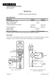
Here you have the <strong>Kalman</strong> <strong>Filter</strong>: (The formulas (8.35) — (8.37) below are<br />
represented by the block diagram shown in Figure 8.1.)<br />
<strong>Kalman</strong> <strong>Filter</strong> state <strong>estimation</strong>:<br />
1. This step is the initial step, and the operations here are executed only<br />
once. Assume that the initial guess of the state is x init . The initial<br />
value x p (0) of the predicted state estimate x p (which is calculated<br />
continuously as described below) is set equal to this initial value:<br />
Initial state estimate<br />
x p (0) = x init (8.34)<br />
2. Calculate the predicted measurement estimate from the predicted<br />
state estimate:<br />
Predicted measurement estimate:<br />
y p (k) =g [x p (k)] (8.35)<br />
(It is assumed that the noise terms Hv(k) and w(k) are not known or<br />
are unpredictable (since they are white noise), so they can not be<br />
used in the calculation of the predicted measurement estimate.)
F. Haugen: Kompendium for Kyb. 2 ved Høgskolen i Oslo 109<br />
3. Calculate the so-called innovation process or variable – it is actually<br />
the measurement estimate error – as the difference between the<br />
measurement y(k) and the predicted measurement y p (k):<br />
Innovation variable:<br />
e(k) =y(k) − y p (k) (8.36)<br />
4. Calculate the corrected state estimate x c (k) by adding the corrective<br />
term Ke(k) to the predicted state estimate x p (k):<br />
Corrected state estimate:<br />
x c (k) =x p (k)+Ke(k) (8.37)<br />
Here, K is the <strong>Kalman</strong> <strong>Filter</strong> gain. The calculation of K is described<br />
below.<br />
Note: Itisx c (k) that is used as the state estimate in applications 1 .<br />
About terminology: The corrected estimate is also denoted the<br />
posteriori estimate because it is calculated after the present<br />
measurement is taken. It is also denoted the measurement-updated<br />
estimate.<br />
Due to the measurement-based correction term of the <strong>Kalman</strong> <strong>Filter</strong>,<br />
you can except the errors of the state estimates to be smaller than if<br />
there were no such correction term. This correction can be regarded<br />
as a feedback correction of the estimates, and it is well known from<br />
dynamic system theory, and in particular control systems theory,<br />
that feedback from measurements reduces errors. This feedback is<br />
indicated in Figure 8.1.<br />
5. Calculate the predicted state estimate for the next time step,<br />
x p (k +1), using the present state estimate x c (k) and the known<br />
input u(k) in process model:<br />
Predicted state estimate:<br />
x p (k +1)=f[x c (k), u(k)] (8.38)<br />
(It is assumed that the noise term Gv(k) is not known or is<br />
unpredictable, since it is random, so it can not be used in the<br />
calculation of the state estimate.)<br />
About terminology: The predicted estimate is also denoted the priori<br />
estimate because it is calculated before the present measurement is<br />
taken. It is also denoted the time-updated estimate.
F. Haugen: Kompendium for Kyb. 2 ved Høgskolen i Oslo 110<br />
Real system (process)<br />
Process noise<br />
(disturbances)<br />
w(k)<br />
(Commonly no connection)<br />
Measurement<br />
noise<br />
v(k)<br />
u(k)<br />
Known inputs<br />
(control variables<br />
and disturbances)<br />
Process<br />
x(k)<br />
x(k+1) = f[x(k),u(k)] + Gw(k)<br />
(Commonly no connection)<br />
<strong>State</strong> variable<br />
(unknown value)<br />
Sensor<br />
y(k) = g[x(k),u(k)]<br />
+ Hw(k) + v(k)<br />
Measurement<br />
variable<br />
y(k)<br />
(Commonly no connection)<br />
<strong>Kalman</strong> <strong>Filter</strong><br />
f()<br />
System<br />
function<br />
x p (k+1)<br />
1/z<br />
Corrected<br />
estimate<br />
x c (k)<br />
Unit<br />
delay<br />
x c (k)<br />
x p (k)<br />
Predicted<br />
estimate<br />
Applied state<br />
estimate<br />
Ke(k)<br />
g()<br />
K<br />
y p (k)<br />
Measurement<br />
function<br />
<strong>Kalman</strong> gain<br />
e(k)<br />
Innovation<br />
variable<br />
or ”process”<br />
Feedback<br />
correction<br />
of estimate<br />
Figure 8.1: The <strong>Kalman</strong> <strong>Filter</strong> algorithm (8.35) — (8.38) represented by a block<br />
diagram<br />
(8.35) — (8.38) can be represented by the block diagram shown in Figure<br />
8.1.<br />
The <strong>Kalman</strong> <strong>Filter</strong> gain is a time-varying gain matrix. It is given by the<br />
algorithm presented below. In the expressions below the following matrices<br />
are used:<br />
• Auto-covariance matrix (for lag zero) of the <strong>estimation</strong> error of the<br />
corrected estimate:<br />
P c = R ex c (0) = E n(x − m xc )(x − m xc ) T o (8.39)<br />
1 Therefore, I have underlined the formula.
F. Haugen: Kompendium for Kyb. 2 ved Høgskolen i Oslo 111<br />
• Auto-covariance matrix (for lag zero) of the <strong>estimation</strong> error of the<br />
predicted estimate:<br />
n<br />
o<br />
P d = R exd (0) = E (x − m xd )(x − m xd ) T (8.40)<br />
• The transition matrix A of a linearized model of the original<br />
nonlinear model (8.14) calculated <strong>with</strong> the most recent state<br />
estimate, which is assumed to be the corrected estimate x c (k):<br />
A = ∂f(·)<br />
¯<br />
∂x<br />
¯xc (k),u(k)<br />
(8.41)<br />
• The measurement gain matrix C of a linearized model of the original<br />
nonlinear model (8.15) calculated <strong>with</strong> the most recent state<br />
estimate:<br />
C = ∂g(·)<br />
¯<br />
(8.42)<br />
∂x<br />
¯xc(k),u(k)<br />
However, it is very common that C = g(), and in these cases no<br />
linearization is necessary.<br />
The <strong>Kalman</strong> <strong>Filter</strong> gain is calculated as follows (these calculations are<br />
repeated each program cycle):<br />
<strong>Kalman</strong> <strong>Filter</strong> gain:<br />
1. This step is the initial step, and the operations here are executed<br />
only once. The initial value P p (0) can be set to some guessed value<br />
(matrix), e.g. to the identity matrix (of proper dimension).<br />
2. Calculation of the <strong>Kalman</strong> Gain:<br />
<strong>Kalman</strong> <strong>Filter</strong> gain:<br />
K(k) =P p (k)C T [CP p (k)C T + R] −1 (8.43)<br />
3. Calculation of auto-covariance of corrected state estimate error:<br />
Auto-covariance of corrected state estimate error:<br />
P c (k) =[I − K(k)C] P p (k) (8.44)<br />
4. Calculation of auto-covariance of the next time step of predicted state<br />
estimate error:<br />
Auto-covariance of predicted state estimate error:<br />
P p (k +1)=AP c (k)A T + GQG T (8.45)
F. Haugen: Kompendium for Kyb. 2 ved Høgskolen i Oslo 112<br />
Here are comments to the <strong>Kalman</strong> <strong>Filter</strong> algorithm presented above:<br />
1. Order of formulas in the program cycle: The <strong>Kalman</strong> <strong>Filter</strong><br />
formulas can be executed in the following order:<br />
• (8.43), <strong>Kalman</strong> <strong>Filter</strong> gain<br />
• (8.36), innovation process (variable)<br />
• (8.37), corrected state estimate, which is the state estimate to be<br />
used in applications<br />
• (8.38), predicted state estimate of next time step<br />
• (8.44), auto-covarience of error of corrected estimate<br />
• (8.41),transitionmatrixinlinearmodel<br />
• (8.42), measurement matrix in linear model<br />
• (8.45), auto-covarience of error of predicted estimate of next<br />
time step<br />
2. Steady-state <strong>Kalman</strong> <strong>Filter</strong> gain. If the model is linear and time<br />
invariant (i.e. system matrices are not varying <strong>with</strong> time) the<br />
auto-covariances P c and P p will converge towards steady-state values.<br />
Consequently, the <strong>Kalman</strong> <strong>Filter</strong> gain will converge towards a<br />
steady-state <strong>Kalman</strong> <strong>Filter</strong> gain value, K 2 s ,whichcanbe<br />
pre-calculated. It is quite common to use only the steady-state gain<br />
in applications.<br />
For a nonlinear system K s may vary <strong>with</strong> the operating point (if the<br />
system matrix A of the linearized model varies <strong>with</strong> the operating<br />
point). In practical applications K s may be re-calculated as the<br />
operating point changes.<br />
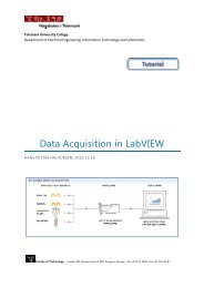
Figure 8.2 illustrates the information needed to compute the<br />
steady-state <strong>Kalman</strong> <strong>Filter</strong> gain, K s .<br />
3. Model errors. There are always model errors since no model can<br />
give a perfect description of a real (practical system). It is possible to<br />
analyze the implications of the model errors on the state estimates<br />
calculated by the <strong>Kalman</strong> <strong>Filter</strong>, but this will not be done in this<br />
book. However, in general, the <strong>estimation</strong> errors are smaller <strong>with</strong> the<br />
<strong>Kalman</strong> <strong>Filter</strong> than <strong>with</strong> a so-called ballistic state estimator, whichis<br />
the state estimator that you get if the <strong>Kalman</strong> <strong>Filter</strong> gain K is set to<br />
zero. In the latter case there is no correction of the estimates. It is<br />
only the predictions (8.38) that make up the estimates. The <strong>Kalman</strong><br />
<strong>Filter</strong> then just runs as a simulator.<br />
2 MATLAB and LabVIEW have functions for calculating the steady-state <strong>Kalman</strong> Gain.
F. Haugen: Kompendium for Kyb. 2 ved Høgskolen i Oslo 113<br />
Transition matrix<br />
Process noise gain matrix<br />
Measurement gain matrix<br />
Process noise auto-covariance<br />
Measurement noise auto -covariance<br />
A<br />
G<br />
C<br />
Q<br />
R<br />
Steady state<br />
<strong>Kalman</strong><br />
<strong>Filter</strong> gain<br />
K s<br />
K s<br />
Figure 8.2: Illustration of what information is needed to compute the steadystate<br />
<strong>Kalman</strong> <strong>Filter</strong> gain, K s .<br />
Note that you can try to estimate model errors by augmenting the<br />
states <strong>with</strong> states representing the model errors. Augmented <strong>Kalman</strong><br />
<strong>Filter</strong> is described in Section 8.4.<br />
4. How to tune the <strong>Kalman</strong> <strong>Filter</strong>: Usually it is necessary to<br />
fine-tune the <strong>Kalman</strong> <strong>Filter</strong> when it is connected to the real system.<br />
The process disturbance (noise) auto-covariance Q and/or the<br />
measurement noise auto-covariance R arecommonlyusedforthe<br />
tuning. However, since R is relatively easy to calculate from a time<br />
series of measurements (using some variance function in for example<br />
LabVIEW or MATLAB), we only consider adjusting Q here.<br />
What is good behaviour of the <strong>Kalman</strong> <strong>Filter</strong> How can good<br />
behaviour be observed It is when the estimates seems to have<br />
reasonable values as you judge from your physical knowledge about<br />
the physical process. In addition the estimates must not be too<br />
noisy! What is the cause of the noise In real systems it is mainly<br />
the measurement noise that introduces noise into the estimates. How<br />
do you tune Q to avoid too noisy estimates The larger Q the<br />
stronger measurement-based updating of the state estimates because<br />
a large Q tells the <strong>Kalman</strong> <strong>Filter</strong> that the variations in the real state<br />
variables are assumed to be large (remember that the process noise<br />
influences on the state variables, cf. (8.15)). Hence, the larger Q the<br />
larger <strong>Kalman</strong> Gain K and the stronger updating of the estimates.<br />
But this causes more measurement noise to be added to the<br />
estimates because the measurement noise is a term in the innovation<br />
process e which is calculated by K:<br />
x c (k) = x p (k)+Ke(k) (8.46)<br />
= x p (k)+K {g [x(k)] + v(k) − g [x p (k)]} (8.47)<br />
where v is real measurement noise. So, the main tuning rule is as<br />
follows: Select as large Q as possible <strong>with</strong>out the state estimates<br />
becoming too noisy.
F. Haugen: Kompendium for Kyb. 2 ved Høgskolen i Oslo 114<br />
But Q is a matrix! How to select it “large” or “small”. Since each of<br />
the process disturbances typically are assumed to act on their<br />
respective state independently, Q can be set as a diagonal matrix:<br />
⎡<br />
⎤<br />
Q 11 0 0 0<br />
0 Q 22 0 0<br />
Q = ⎢<br />
⎣<br />
.<br />
0 0 ..<br />
⎥<br />
0 ⎦ = diag(Q 11,Q 22 , ··· ,Q nn ) (8.48)<br />
0 0 0 Q nn<br />
where each of the diagonal elements can be adjusted independently.<br />
If you do not have any idea about numerical values, you can start by<br />
setting all the diagonal elements to one, and hence Q is<br />
⎡<br />
⎤<br />
1 0 0 0<br />
0 1 0 0<br />
Q = Q 0 ⎢<br />
⎣ 0 0 . .<br />
⎥<br />
(8.49)<br />
. 0 ⎦<br />
0 0 0 1<br />
where Q 0 is the only tuning parameter. If you do not have any idea<br />
about a proper value of Q 0 you may initially try<br />
Q 0 =0.01 (8.50)<br />
Then you may adjust Q 0 or try to fine tune each of the diagonal<br />
elements individually.<br />
5. The error-model: Assuming that the system model is linear and<br />
that the model is correct (giving a correct representation of the real<br />
system), it can be shown that the behaviour of the error of the<br />
corrected state <strong>estimation</strong>, e xc (k), cf. (8.13), is given by the following<br />
error-model: 3<br />
Error-model of <strong>Kalman</strong> <strong>Filter</strong>:<br />
e xc (k +1)=(I − KC) Ae xc (k)+(I − KC) Gv(k) − Kw(k +1)<br />
(8.51)<br />
This model can be used to analyze the <strong>Kalman</strong> <strong>Filter</strong>.<br />
Note: (8.13) is not identical to the auto-covariance of the <strong>estimation</strong><br />
error which is<br />
P c (k) =E{[e xc (k) − m xc (k)][e xc (k) − m xc (k)] T } (8.52)<br />
But (8.13) is the trace of P c (the trace is the sum of the diagonal<br />
elements):<br />
e xc = trace [ P c (k)] (8.53)<br />
3 You can derive this model by subtracting the model describing the corrected state<br />
estimate from the model that describes the real state (the latter is simply the process<br />
model).
F. Haugen: Kompendium for Kyb. 2 ved Høgskolen i Oslo 115<br />
6. The dynamics of the <strong>Kalman</strong> <strong>Filter</strong>. The error-model (8.51) of<br />
the <strong>Kalman</strong> <strong>Filter</strong> represents a dynamic system. The dynamics of the<br />
<strong>Kalman</strong> <strong>Filter</strong> is given can be analyzed by calculating the eigenvalues<br />
of the system matrix of (8.51). These eigenvalues are<br />
{λ 1 ,λ 2 ,...,λ n } = eig [(I − KC)A] (8.54)<br />
7. The stability of the <strong>Kalman</strong> <strong>Filter</strong>. It can be shown that the<br />
<strong>Kalman</strong> <strong>Filter</strong> always is an asymptotically stable dynamic system<br />
(otherwise it could not give an optimal estimate). In other words,<br />
the eigenvalues defined by (8.54) are always inside the unity circle.<br />
8. Testing the <strong>Kalman</strong> <strong>Filter</strong> before practical use: As<strong>with</strong>every<br />
model-based algorithm (as controllers) you should test your <strong>Kalman</strong><br />
<strong>Filter</strong> <strong>with</strong> a simulated process before applying it to the real system.<br />
You can implement a simulator in e.g. LabVIEW or<br />
MATLAB/Simulink since you already have a model (the <strong>Kalman</strong><br />
<strong>Filter</strong> is model-based).<br />
Firstly, you should test the <strong>Kalman</strong> <strong>Filter</strong> <strong>with</strong> the nominal model in<br />
the simulator, including process and measurement noise. This is the<br />
model that you are basing the <strong>Kalman</strong> <strong>Filter</strong> on. Secondly, you<br />
should introduce some reasonable model errors by making the<br />
simulator model somewhat different from the <strong>Kalman</strong> <strong>Filter</strong> model,<br />
and observe if the <strong>Kalman</strong> <strong>Filter</strong> still produces usable estimates.<br />
9. Predictor type <strong>Kalman</strong> <strong>Filter</strong>. In the predictortypeofthe<br />
<strong>Kalman</strong> <strong>Filter</strong> there is only one formula for the calculation of the<br />
state estimate:<br />
x est (k +1)=Ax est (k)+K[y(k) − Cx est (k)] (8.55)<br />
Thus, there is no distinction between the predicted state estimate<br />
and the corrected estimate (it the same variable). (Actually, this is<br />
the original version of the <strong>Kalman</strong> <strong>Filter</strong>[7].) The predictor type<br />
<strong>Kalman</strong> <strong>Filter</strong> has the drawback that there is a time delay of one<br />
time step between the measurement y(k) and the calculated state<br />
estimate x est (k +1).<br />
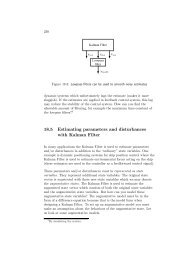
8.4 Estimating parameters and disturbances <strong>with</strong><br />
<strong>Kalman</strong> <strong>Filter</strong><br />
In many applications the <strong>Kalman</strong> <strong>Filter</strong> is used to estimate parameters<br />
and/or disturbances in addition to the “ordinary” state variables. One
F. Haugen: Kompendium for Kyb. 2 ved Høgskolen i Oslo 116<br />
example is dynamic positioning systems for ship position control where the<br />
<strong>Kalman</strong> <strong>Filter</strong> is used to estimate environmental forces acting on the ship<br />
(these estimates are used in the controller as a feedforward control signal).<br />
These parameters and/or disturbances must be represented as state<br />
variables. They represent additional state variables. The original state<br />
vector is augmented <strong>with</strong> these new state variables which we may denote<br />
the augmentative states. The <strong>Kalman</strong> <strong>Filter</strong> is used to estimate the<br />
augmented state vector which consists of both the original state variables<br />
and the augmentative state variables. But how can you model these<br />
augmentative state variables The augmentative model must be in the<br />
form of a difference equation because that is the model form of state<br />
variables are defined. To set up an augmentative model you must make an<br />
assumption about the behaviour of the augmentative state. Let us look at<br />
some augmentative models.<br />
• Augmentative state is (almost) constant: The most common<br />
augmentative model is based on the assumption that the<br />
augmentative state variable x a is slowly varying, almost constant.<br />
The corresponding differential equation is<br />
ẋ a (t) =0 (8.56)<br />
Discretizing this differential equation <strong>with</strong> the Euler Forward method<br />
gives<br />
x a (k +1)=x a (k) (8.57)<br />
which is a difference equation ready for <strong>Kalman</strong> <strong>Filter</strong> algorithm. It<br />
is however common to assume that the state is driven by some noise,<br />
hence the augmentative model become:<br />
x a (k +1)=x a (k)+w a (k) (8.58)<br />
where w a is white process noise <strong>with</strong> assumed auto-covariance on the<br />
form R wa (L) =Q a δ(L). As pointed out in Section 8.3, the variance<br />
Q a can be used as a tuning parameter of the <strong>Kalman</strong> <strong>Filter</strong>.<br />
• Augmentative state has (almost) constant rate: The<br />
corresponding differential equation is<br />
or, in state space form, <strong>with</strong> x a1 ≡ x a ,<br />
ẍ a =0 (8.59)<br />
ẋ a1 = x a2 (8.60)<br />
ẋ a2 =0 (8.61)
F. Haugen: Kompendium for Kyb. 2 ved Høgskolen i Oslo 117<br />
where x a2 is another augmentative state variable. Applying Euler<br />
Forward discretization <strong>with</strong> sampling interval h [sec] to (8.60) —<br />
(8.61) and including white process noise to the resulting difference<br />
equations gives<br />
x a1 (k +1)=x a1 (k)+hx a2 (k)+w a1 (k) (8.62)<br />
x a2 (k +1)=x a2 (k)+w a2 (k) (8.63)<br />
Once you have defined the augmented model, you can design and<br />
implement the <strong>Kalman</strong> <strong>Filter</strong> in the usual way. The <strong>Kalman</strong> <strong>Filter</strong> then<br />
estimates both the original states and the augmentative states.<br />
The following example shows how the state augementation can be done in<br />
a practical application. The example also shows how to use functions in<br />
LabVIEW and in MATLAB to calculate the steady state <strong>Kalman</strong> <strong>Filter</strong><br />
gain.<br />
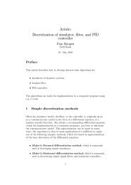
Example 19 <strong>Kalman</strong> <strong>Filter</strong><br />
Figure 8.3 shows a liquid tank. We will design a steady state <strong>Kalman</strong><br />
<strong>Filter</strong> to estimate the outflow F out .Thelevelh is measured.<br />
Mass balance of the liquid in the tank is (mass is ρAh)<br />
ρA tank ḣ(t) = ρK p u − ρF out (t) (8.64)<br />
= ρK p u − ρF out (t) (8.65)<br />
After cancelling the density ρ the model is<br />
ḣ(t) = 1<br />
A tank<br />
[K p u − F out (t)] (8.66)<br />
We assume that the unknown outflow is slowly changing, almost constant.<br />
We define the following augmentative model:<br />
˙ F out (t) =0 (8.67)<br />
The model of the system is given by (8.66) — (8.67). Although it is not<br />
necessary, it is convenient to rename the state variables using standard<br />
names. So we define<br />
x 1 = h (8.68)<br />
x 2 = F out (8.69)
F. Haugen: Kompendium for Kyb. 2 ved Høgskolen i Oslo 118<br />
u [V]<br />
K p [m 3 /V]<br />
F in [m 3 /s]<br />
h [m]<br />
0<br />
A [m 2 ]<br />
F out [m 3 /s]<br />
Level<br />
sensor<br />
m [kg]<br />
[kg/m 3 ]<br />
Measured<br />
h [m]<br />
<strong>Kalman</strong><br />
<strong>Filter</strong><br />
Estimated<br />
F out<br />
Figure 8.3: Example 19: Liquid tank<br />
The model (8.66) — (8.67) is now<br />
ẋ 1 (t) = 1 [K p u(t) − x 2 (t)] (8.70)<br />
A tank<br />
ẋ 2 (t) =0 (8.71)<br />
Applying Euler Forward discretization <strong>with</strong> time step T and including<br />
white disturbance noise in the resulting difference equations yields<br />
x 1 (k +1)=x 1 (k)+<br />
T [K p u(k) − x 2 (k)] + w 1 (k) (8.72)<br />
A<br />
| tank<br />
{z }<br />
f 1 (·)<br />
x 2 (k +1)=x 2 (k) + w<br />
| {z } 2 (k) (8.73)<br />
f 2 (·)<br />
or<br />
x(k +1)=f [x(k),u(k)] + w(k) (8.74)<br />
w 1 and w 2 are independent (uncorrelated) white process noises <strong>with</strong><br />
assumed variances R w1 (L) =Q 1 δ(L) and R w2 (L) =Q 2 δ(L) respectively.<br />
Here, Q 1 and Q 2 are variances. The multivariable noise model is then<br />
· ¸<br />
w1<br />
w =<br />
(8.75)<br />
w 2
F. Haugen: Kompendium for Kyb. 2 ved Høgskolen i Oslo 119<br />
<strong>with</strong> auto-covariance<br />
where<br />
R w (L) =Qδ(L) (8.76)<br />
Q =<br />
· ¸<br />
Q11 0<br />
0 Q 22<br />
(8.77)<br />
Assuming that the level x 1 is measured, we add the following measurement<br />
equation to the state space model:<br />
y(k) =g [x p (k),u(k)] + v(k) =x 1 (k)+v(k) (8.78)<br />
where v is white measurement noise <strong>with</strong> assumed variance<br />
where R is the measurement variance.<br />
The following numerical values are used:<br />
R v (L) =Rδ(L) (8.79)<br />
Sampling time: T =0.1 s (8.80)<br />
A tank =0.1 m 2 (8.81)<br />
K p =0.001 (m 3 /s)/V (8.82)<br />
· ¸<br />
0.01 0<br />
Q =<br />
(initally, may be adjusted)<br />
0 0.01<br />
(8.83)<br />
R =0.0001 m 2 (Gaussian white noise) (8.84)<br />
We will set the initial estimates as follows:<br />
x 1p (0) = x 1 (0) = y(0) (from the sensor) (8.85)<br />
x 2p (0) = 0 (assuming no information about initial value (8.86)<br />
The <strong>Kalman</strong> <strong>Filter</strong> algorithm is as follows: The predicted level<br />
measurement is calculated according to (8.35):<br />
y p (k) =g [x p (k),u(k)] = x 1p (k) (8.87)<br />
<strong>with</strong> initial value as given by (8.85). The innovation variable is calculated<br />
according to (8.36), where y is the level measurement:<br />
e(k) =y(k) − y p (k) (8.88)<br />
The corrected state estimate is calculated according to (8.37):<br />
x c (k) =x p (k)+Ke(k) (8.89)
F. Haugen: Kompendium for Kyb. 2 ved Høgskolen i Oslo 120<br />
or, in detail:<br />
·<br />
x1c (k)<br />
x 2c (k)<br />
This is the applied esimate!<br />
¸<br />
=<br />
·<br />
x1p (k)<br />
x 2p (k)<br />
¸<br />
· ¸<br />
K11<br />
+ e(k) (8.90)<br />
K 21<br />
| {z }<br />
K<br />
Thepredictedstateestimateforthenexttimestep,x p (k +1), is calculated<br />
accordingto(8.38):<br />
x p (k +1)=f[x c (k), u(k)] (8.91)<br />
or, in detail:<br />
·<br />
x1p (k +1)<br />
x 2p (k +1)<br />
¸<br />
=<br />
· ¸ ·<br />
f1 x1c (k)+<br />
=<br />
A T<br />
tank<br />
[K p u(k) − x 2c (k)]<br />
f 2 x 2c (k)<br />
¸<br />
(8.92)<br />
To calculate the steady state <strong>Kalman</strong> <strong>Filter</strong> gain K s the following<br />
information is needed, cf. Figure 8.2:<br />
A = ∂f(·)<br />
¯<br />
∂x<br />
¯xp(k),u(k)<br />
⎡<br />
⎤<br />
∂f 1 ∂f 1<br />
∂x<br />
⎢ 1 ∂x 2<br />
⎥<br />
= ⎣<br />
⎦¯<br />
Q =<br />
G =<br />
=<br />
⎡<br />
⎣<br />
· 1 0<br />
0 1<br />
· 0.01 0<br />
0 0.01<br />
∂f 2<br />
∂x 1<br />
∂f 2<br />
∂x 2<br />
1 − T<br />
A tank<br />
0 1<br />
¯<br />
¯xp (k),u(k)<br />
⎤<br />
(8.93)<br />
(8.94)<br />
⎦ (8.95)<br />
¸<br />
= I 2 (identity matrix) (8.96)<br />
C = ∂g(·)<br />
¯<br />
(8.97)<br />
∂x<br />
¯xp (k),u(k)<br />
= £ 1 0 ¤ (8.98)<br />
¸<br />
(initially, may be adjusted) (8.99)<br />
R =0.001 m 2 (8.100)<br />
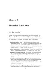
Figure 8.4 shows the front panel of a LabVIEW simulator of this example.<br />
The outflow F out = x 2 was changed during the simulation, and the <strong>Kalman</strong><br />
<strong>Filter</strong> estimates the correct steady state value (the estimate is however
F. Haugen: Kompendium for Kyb. 2 ved Høgskolen i Oslo 121<br />
Figure 8.4: Example 19: Front panel of a LabVIEW simulator of this example<br />
noisy). During the simulations, I found that (8.99) gave too noise estimate<br />
of x 2 = F out . I ended up <strong>with</strong><br />
· ¸<br />
0.01 0<br />
Q =<br />
0 10 −6 (8.101)<br />
as a proper value.<br />
Figure 8.5 shows how the steady state <strong>Kalman</strong> <strong>Filter</strong> gain K s is calculated<br />
using the <strong>Kalman</strong> Gain function. The figure also shows how to check for<br />
observability <strong>with</strong> the Observability Matrix function. Figure 8.6 shows<br />
the implementation of the <strong>Kalman</strong> <strong>Filter</strong> equations in a Formula Node.<br />
Below is MATLAB code that calculates the steady state <strong>Kalman</strong> <strong>Filter</strong><br />
gain. It is calculated <strong>with</strong> the dlqe 4 function (in Control System Toolbox).<br />
A=[1,-1;0,1]<br />
G=[1,0;0,1]<br />
C=[1,0]<br />
4 dlqe = Discrete-time linear quadratic estimator.
F. Haugen: Kompendium for Kyb. 2 ved Høgskolen i Oslo 122<br />
Figure 8.5: Example 19: Calculation of the steady state <strong>Kalman</strong> <strong>Filter</strong> gain <strong>with</strong><br />
the <strong>Kalman</strong> Gain function, and checking for observability <strong>with</strong> the Observability<br />
Matrix function.<br />
Q=[0.01,0;0,1e-6]<br />
R=[0.0001];<br />
[K,Pp,Pc,E] = dlqe(A,G,C,Q,R)<br />
K is the steady state <strong>Kalman</strong> <strong>Filter</strong> gain. (Pp and Pc are steady state<br />
<strong>estimation</strong> error auto-covariances, cf. (8.45) and (8.44). E is a vector<br />
containing the eigenvalues of the <strong>Kalman</strong> <strong>Filter</strong>, cf. (8.54).)<br />
MATLAB answers<br />
K =<br />
0.9903<br />
-0.0099<br />
Which is the same as calculated by the LabVIEW function <strong>Kalman</strong><br />
Gain, cf. Figure 8.5.
F. Haugen: Kompendium for Kyb. 2 ved Høgskolen i Oslo 123<br />
Figure 8.6: Example 19: Implementation of the <strong>Kalman</strong> <strong>Filter</strong> equations in a<br />
Formula Node. (The <strong>Kalman</strong> <strong>Filter</strong> gain is fetched from the While loop in the<br />
Block diagram using local variables.)<br />
[End of Example 19]<br />
8.5 <strong>State</strong> estimators for deterministic systems:<br />
Observers<br />
Assume that the system (process) for which we are to calculate the state<br />
estimate has no process disturbances:<br />
and no measurement noise signals:<br />
w(k) ≡ 0 (8.102)<br />
v(k) ≡ 0 (8.103)<br />
Then the system is not a stochastic system any more. In stead we can say<br />
is is non-stochastic or deterministic. Anobserver is a state estimator for a<br />
deterministic system. It is common to use the same estimator formulas in
F. Haugen: Kompendium for Kyb. 2 ved Høgskolen i Oslo 124<br />
an observer as in the <strong>Kalman</strong> <strong>Filter</strong>, namely (8.35), (8.36), (8.37) and<br />
(8.38). For convenience these formulas are repeated here:<br />
Predicted measurement estimate:<br />
y p (k) =g [x p (k)] (8.104)<br />
Innovation variable:<br />
e(k) =y(k) − y p (k) (8.105)<br />
Corrected state estimate:<br />
x c (k) =x p (k)+Ke(k) (8.106)<br />
Predicted state estimate:<br />
x p (k +1)=f[x c (k), u(k)] (8.107)<br />
The estimator gain K (corresponding to the <strong>Kalman</strong> <strong>Filter</strong> gain in the<br />
stochastic case) is calculated from a specification of the eigenvalues of the<br />
error-model of the observer. The error-model is given by (8.51) <strong>with</strong><br />
w(k) =0and v(k) =0,hence:<br />
Error-model of observers:<br />
e xc (k +1)=(I − KC) Ae | {z }<br />
xc (k) =A e e xc (k) (8.108)<br />
A e<br />
where A e is the transition matrix of the error-model. The error-model<br />
shows how the state <strong>estimation</strong> error develops as a function of time from<br />
an initial error e xc (0). If the error-model is asymptotically stable, the<br />
steady-state <strong>estimation</strong> errors will be zero (because (8.108) is an<br />
autonomous system.) The dynamic behaviour of the <strong>estimation</strong> errors is<br />
given by the eigenvalues of the transition matrix A e (8.108).<br />
But how to calculate a proper value of the estimator gain K Wecanno<br />
longer use the formulas (8.43) — (8.45). In stead, K can be calculated from<br />
the specified eigenvalues {z 1 ,z 2 ,...,z n } of A e :<br />
eig [A e ]=eig [(I − KC) A] ={z 1 ,z 2 ,...,z n } (8.109)<br />
As is known from mathematics, the eigenvalues are the λ-roots of the<br />
characteristic equation:<br />
det [zI − (I − KC) A] =(z − z 1 )(z − z 2 ) ···(z − z n )=0 (8.110)<br />
In (8.110) all terms except K are known or specified. To actually calculate<br />
K from (8.109) you should use computer tools as Matlab or LabVIEW. In
F. Haugen: Kompendium for Kyb. 2 ved Høgskolen i Oslo 125<br />
Matlab you can use the function place (in Control System Toobox). In<br />
LabVIEW you can use the function CD Place.vi (in Control Design<br />
Toolkit), and in MathScript (LabVIEW) you can use place. But how to<br />
specify the eigenvalues {z i } One possibility is to specify discrete-time<br />
Butterworth eigenvalues {z i }. Alternatively you can specify<br />
continuous-time eigenvalues {s i } which you transform to discrete-time<br />
eigenvalues using the transformation<br />
z i = e s ih<br />
(8.111)<br />
where h [s] is the time step.<br />
Example 20 Calculating the observer gain K<br />
The following MathScript-script or Matlab-script calculates the estimator<br />
gain K using the place function. Note that place calculates the gain K 1<br />
so that the eigenvalues of the matrix (A 1 − B 1 K 1 ) are as specified. place<br />
is used as follows:<br />
K=place(A,B,z)<br />
But we need to calculate K so that the eigenvalues of (I − KC) A =<br />
A − KCA are as specified. The eigenvalues of A − KCA are the same as<br />
the eigenvalues of<br />
Therefore we must use place as follows:<br />
K1=place(A’,(C*A)’,z);<br />
K=K1’<br />
Here is the script:<br />
(A − KCA) T = A T − (AC) T K T (8.112)<br />
h=0.05; %Time step<br />
s=[-2+2j, -2-2j]’; %Specified s-eigenvalues<br />
z=exp(s*h); %Corresponding z-eigenvalues<br />
A = [1,0.05;0,0.95]; %Transition matrix<br />
B = [0;0.05]; %Input matrix<br />
C = [1,0]; %Output matrix<br />
D = [0]; %Direct-output matrix<br />
K1=place(A’,(C*A)’,z); %Calculating gain K1 using place<br />
K=K1’ %Transposing K<br />
The result is
F. Haugen: Kompendium for Kyb. 2 ved Høgskolen i Oslo 126<br />
K =<br />
0.13818<br />
0.22376<br />
The function CD Place.vi on the Control Design Toolkit palette in<br />
LabVIEW can also be used to calculate the estimator gain K. Figure 8.7<br />
shows the front panel and Figure 8.8 shows the block diagram of a<br />
LabVIEW program that calculates K for the same system as above. The<br />
same K is obtained.<br />
Figure 8.7: Example 20: Front panel of the LabVIEW program to calculate the<br />
estimator gain K<br />
Figure 8.8: Example 20: Block diagram of the LabVIEW program to calculate<br />
the estimator gain K<br />
[End of Example 20]
F. Haugen: Kompendium for Kyb. 2 ved Høgskolen i Oslo 127<br />
8.6 <strong>Kalman</strong> <strong>Filter</strong> or Observer<br />
Now you have seen two ways to calculate the estimator gain K of a state<br />
estimator:<br />
• K is the <strong>Kalman</strong> Gain in a <strong>Kalman</strong> <strong>Filter</strong><br />
• K is the estimator gain in an observer<br />
The formulas for calculating the state estimate are the same in both cases:<br />
• <strong>Kalman</strong> <strong>Filter</strong>: (8.35), (8.36), (8.37), (8.38).<br />
• Observer: (8.104), (8.105), (8.106), (8.107).<br />
The observer may seem simpler than the <strong>Kalman</strong> <strong>Filter</strong>, but there is a<br />
potential danger in using the observer: The observer does not calculate<br />
any optimal state estimate in the least mean square sense, and hence the<br />
state estimate may become too noisy due to the inevitable measurement<br />
noise if you specify too fast error models dynamics (i.e. too large absolute<br />
value of the error-model eigenvalues). This is because fast dynamics<br />
requires a large estimator gain K, causing the measurement noise to give<br />
large influence on the state estimates. In my opinion, the <strong>Kalman</strong> <strong>Filter</strong><br />
gives a better approach to state <strong>estimation</strong> because it is easier and more<br />
intuitive to tune the filter in terms of process and measurement noise<br />
variances than in terms of eigenvalues of the error-model.