State estimation with Kalman Filter

More documents

Recommendations

Info

F. Haugen: Kompendium for Kyb. 2 ved Høgskolen i Oslo 112 Here are comments to the Kalman Filter algorithm presented above: 1. Order of formulas in the program cycle: The Kalman Filter formulas can be executed in the following order: • (8.43), Kalman Filter gain • (8.36), innovation process (variable) • (8.37), corrected state estimate, which is the state estimate to be used in applications • (8.38), predicted state estimate of next time step • (8.44), auto-covarience of error of corrected estimate • (8.41),transitionmatrixinlinearmodel • (8.42), measurement matrix in linear model • (8.45), auto-covarience of error of predicted estimate of next time step 2. Steady-state Kalman Filter gain. If the model is linear and time invariant (i.e. system matrices are not varying with time) the auto-covariances P c and P p will converge towards steady-state values. Consequently, the Kalman Filter gain will converge towards a steady-state Kalman Filter gain value, K 2 s ,whichcanbe pre-calculated. It is quite common to use only the steady-state gain in applications. For a nonlinear system K s may vary with the operating point (if the system matrix A of the linearized model varies with the operating point). In practical applications K s may be re-calculated as the operating point changes. 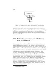Figure 8.2 illustrates the information needed to compute the steady-state Kalman Filter gain, K s . 3. Model errors. There are always model errors since no model can give a perfect description of a real (practical system). It is possible to analyze the implications of the model errors on the state estimates calculated by the Kalman Filter, but this will not be done in this book. However, in general, the estimation errors are smaller with the Kalman Filter than with a so-called ballistic state estimator, whichis the state estimator that you get if the Kalman Filter gain K is set to zero. In the latter case there is no correction of the estimates. It is only the predictions (8.38) that make up the estimates. The Kalman Filter then just runs as a simulator. 2 MATLAB and LabVIEW have functions for calculating the steady-state Kalman Gain.
F. Haugen: Kompendium for Kyb. 2 ved Høgskolen i Oslo 113 Transition matrix Process noise gain matrix Measurement gain matrix Process noise auto-covariance Measurement noise auto -covariance A G C Q R Steady state Kalman Filter gain K s K s Figure 8.2: Illustration of what information is needed to compute the steadystate Kalman Filter gain, K s . Note that you can try to estimate model errors by augmenting the states with states representing the model errors. Augmented Kalman Filter is described in Section 8.4. 4. How to tune the Kalman Filter: Usually it is necessary to fine-tune the Kalman Filter when it is connected to the real system. The process disturbance (noise) auto-covariance Q and/or the measurement noise auto-covariance R arecommonlyusedforthe tuning. However, since R is relatively easy to calculate from a time series of measurements (using some variance function in for example LabVIEW or MATLAB), we only consider adjusting Q here. What is good behaviour of the Kalman Filter How can good behaviour be observed It is when the estimates seems to have reasonable values as you judge from your physical knowledge about the physical process. In addition the estimates must not be too noisy! What is the cause of the noise In real systems it is mainly the measurement noise that introduces noise into the estimates. How do you tune Q to avoid too noisy estimates The larger Q the stronger measurement-based updating of the state estimates because a large Q tells the Kalman Filter that the variations in the real state variables are assumed to be large (remember that the process noise influences on the state variables, cf. (8.15)). Hence, the larger Q the larger Kalman Gain K and the stronger updating of the estimates. But this causes more measurement noise to be added to the estimates because the measurement noise is a term in the innovation process e which is calculated by K: x c (k) = x p (k)+Ke(k) (8.46) = x p (k)+K {g [x(k)] + v(k) − g [x p (k)]} (8.47) where v is real measurement noise. So, the main tuning rule is as follows: Select as large Q as possible without the state estimates becoming too noisy.
Page 1 and 2: Chapter 8 State estimation with Kal
Page 3 and 4: F. Haugen: Kompendium for Kyb. 2 ve
Page 11: F. Haugen: Kompendium for Kyb. 2 ve
Page 27: F. Haugen: Kompendium for Kyb. 2 ve

State estimation with Kalman Filter

You also want an ePaper? Increase the reach of your titles

Delete template?

Save as template?