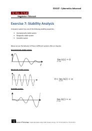
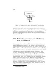
State estimation with Kalman Filter

F. Haugen: Kompendium for Kyb. 2 ved Høgskolen i Oslo 119
with auto-covariance
where
R w (L) =Qδ(L) (8.76)
Q =
· ¸
Q11 0
0 Q 22
(8.77)
Assuming that the level x 1 is measured, we add the following measurement
equation to the state space model:
y(k) =g [x p (k),u(k)] + v(k) =x 1 (k)+v(k) (8.78)
where v is white measurement noise with assumed variance
where R is the measurement variance.
The following numerical values are used:
R v (L) =Rδ(L) (8.79)
Sampling time: T =0.1 s (8.80)
A tank =0.1 m 2 (8.81)
K p =0.001 (m 3 /s)/V (8.82)
· ¸
0.01 0
Q =
(initally, may be adjusted)
0 0.01
(8.83)
R =0.0001 m 2 (Gaussian white noise) (8.84)
We will set the initial estimates as follows:
x 1p (0) = x 1 (0) = y(0) (from the sensor) (8.85)
x 2p (0) = 0 (assuming no information about initial value (8.86)
The Kalman Filter algorithm is as follows: The predicted level
measurement is calculated according to (8.35):
y p (k) =g [x p (k),u(k)] = x 1p (k) (8.87)
with initial value as given by (8.85). The innovation variable is calculated
according to (8.36), where y is the level measurement:
e(k) =y(k) − y p (k) (8.88)
The corrected state estimate is calculated according to (8.37):
x c (k) =x p (k)+Ke(k) (8.89)