State estimation with Kalman Filter
State estimation with Kalman Filter
State estimation with Kalman Filter

You also want an ePaper? Increase the reach of your titles
YUMPU automatically turns print PDFs into web optimized ePapers that Google loves.
F. Haugen: Kompendium for Kyb. 2 ved Høgskolen i Oslo 121<br />
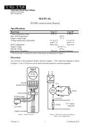
Figure 8.4: Example 19: Front panel of a LabVIEW simulator of this example<br />
noisy). During the simulations, I found that (8.99) gave too noise estimate<br />
of x 2 = F out . I ended up <strong>with</strong><br />
· ¸<br />
0.01 0<br />
Q =<br />
0 10 −6 (8.101)<br />
as a proper value.<br />
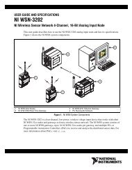
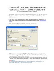
Figure 8.5 shows how the steady state <strong>Kalman</strong> <strong>Filter</strong> gain K s is calculated<br />
using the <strong>Kalman</strong> Gain function. The figure also shows how to check for<br />
observability <strong>with</strong> the Observability Matrix function. Figure 8.6 shows<br />
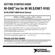
the implementation of the <strong>Kalman</strong> <strong>Filter</strong> equations in a Formula Node.<br />
Below is MATLAB code that calculates the steady state <strong>Kalman</strong> <strong>Filter</strong><br />
gain. It is calculated <strong>with</strong> the dlqe 4 function (in Control System Toolbox).<br />
A=[1,-1;0,1]<br />
G=[1,0;0,1]<br />
C=[1,0]<br />
4 dlqe = Discrete-time linear quadratic estimator.