class lecture notes 10
class lecture notes 10
class lecture notes 10

Create successful ePaper yourself
Turn your PDF publications into a flip-book with our unique Google optimized e-Paper software.
Chapter <strong>10</strong><br />
Hypothesis Tests Regarding a<br />
Parameter<br />
A second type of statistical inference is hypothesis testing. Here, rather than use<br />
either a point (or interval) estimate from a simple random sample to approximate a<br />
population parameter, hypothesis testing uses point estimate to decide which of two<br />
hypotheses (guesses) about parameter is correct. We will look at hypothesis tests for<br />
proportion, p, mean, µ and standard deviation, σ.<br />
<strong>10</strong>.1 The Language of Hypothesis Testing<br />
In this section, we discuss hypothesis testing in general.<br />
Exercise <strong>10</strong>.1(The Language of Hypothesis Testing)<br />
1. Test for binomial proportion, p, right-handed: defective batteries.<br />
In a battery factory, 8% of all batteries made are assumed to be defective.<br />
Technical trouble with production line, however, has raised concern percent<br />
defective has increased in past few weeks. Of n = 600 batteries chosen at<br />
70<br />
random, ths ( 70<br />
≈ 600 600 0.117) of them are found to be defective. Does data<br />
support concern about defective batteries at α = 0.05<br />
(a) Statement. Choose one.<br />
i. H 0 : p = 0.08 versus H 1 : p < 0.08<br />
ii. H 0 : p ≤ 0.08 versus H 1 : p > 0.08<br />
iii. H 0 : p = 0.08 versus H 1 : p > 0.08<br />
(b) Test.<br />
161
162 Chapter <strong>10</strong>. Hypothesis Tests Regarding a Parameter (ATTENDANCE <strong>10</strong>)<br />
Chance ˆp = 70<br />
600 ≈ 0.117 or more, if p 0 = 0.08, is<br />
p–value = P(ˆp ≥ 0.117) = P<br />
⎛<br />
⎝ ˆp−p 0<br />
√<br />
p0 (1−p 0 )<br />
n<br />
which equals (circle one) 0.00 / 0.04 / 4.65.<br />
⎞<br />
≥ 0.117−0.08 √ ⎠ ≈ P (Z ≥ 3.31) ≈<br />
0.08(1−0.08)<br />
600<br />
(Stat, Proportions, One sample, with summary, Number of successes: 70, Number of observations:<br />
600, Next, Null: prop. = 0.08 Alternative: > Calculate.)<br />
Level of significance α = (choose one) 0.01 / 0.05 / 0.<strong>10</strong>.<br />
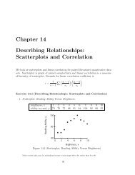
(c) Conclusion.<br />
Since p–value = 0.0005 < α = 0.05,<br />
(circle one) do not reject / reject null guess: H 0 : p = 0.08.<br />
So, sample ˆp indicates population proportion p<br />
is less than / equals / is greater than 0.08: H 1 : p > 0.08.<br />
do not reject null<br />
f<br />
reject null<br />
(critical region)<br />
α = 0.050<br />
p-value = 0.0005<br />
^<br />
p = 0.080 p = 0.117<br />
z = 0<br />
z = 3.31<br />
0<br />
null hypothesis<br />
Figure <strong>10</strong>.1(P-value for sample ˆp = 0.117, if guess p 0 = 0.08)<br />
(d) A comment: null hypothesis and alternative hypothesis.<br />
In this hypothesis test, we are asked to choose between<br />
(choose one) one / two / three alternatives (or hypotheses, or guesses):<br />
a null hypothesis of H 0 : p = 0.08 and an alternative of H 1 : p > 0.08.<br />
Null hypothesis is a statement of “status quo”, of no change; test statistic<br />
used to reject it or not. Alternative hypothesis is “challenger” statement.<br />
(e) Another comment: p-value.<br />
In this hypothesis test, p–value is chance observed proportion defective is<br />
0.117 or more, guessing population proportion defective is p 0 = 0.08 /<br />
p 0 = 0.117.<br />
In general, p-value is probability of observing test statistic or more extreme,<br />
assuming null hypothesis is true.<br />
(f) And another comment: test statistic different for different samples.<br />
If a second sampleof 600 batteries were taken at random fromall batteries,<br />
observed proportion defective of this second group of 600 students would
Section 1. The Language of Hypothesis Testing (ATTENDANCE <strong>10</strong>) 163<br />
probably be (choose one) different from / same as<br />
first observed proportion defective given above, ˆp = 0.117, say, ˆp = 0.09<br />
which may change the conclusions of hypothesis test.<br />
(g) Possible mistake: Type I error.<br />
Even though hypothesis test tells us population proportion defective is<br />
greater than 0.08, that alternative H 1 : p > 0.08 is correct, we could be<br />
wrong. If we were indeed wrong, we should have picked null / alternative<br />
hypothesis H 0 : p = 0.08 instead. Type I error is mistakenly rejecting null.<br />
Also, α = P(type I error).<br />
2. Test p, right–sided again: defective batteries.<br />
54<br />
Of n = 600 batteries chosen at random, ths ( 54<br />
= 600 600 0.09) , instead of 0.117,<br />
of them are found to be defective. Does data support concern about increase<br />
in defective batteries (from 0.08) at α = 0.05 in this case<br />
(a) Statement. Choose one.<br />
i. H 0 : p = 0.08 versus H 1 : p < 0.08<br />
ii. H 0 : p ≤ 0.08 versus H 1 : p > 0.08<br />
iii. H 0 : p = 0.08 versus H 1 : p > 0.08<br />
(b) Test.<br />
Chance ˆp = 54<br />
600 = 0.09 or more, if p 0 = 0.08, is<br />
p–value = P(ˆp ≥ 0.09) = P<br />
⎛<br />
⎝ ˆp−p 0<br />
√<br />
p0 (1−p 0 )<br />
n<br />
which equals (circle one) 0.00 / 0.09 / 0.18.<br />
⎞<br />
≥ 0.09−0.08 ⎠ ≈ P (Z ≥ 0.903) ≈<br />
√ 0.08(1−0.08)<br />
600<br />
(Options, Number of successes: 54, Number of observations: 600, Next, Null: prop. = 0.08 Alternative:<br />
> Calculate.)<br />
Level of significance α = (choose one) 0.01 / 0.05 / 0.<strong>10</strong>.<br />
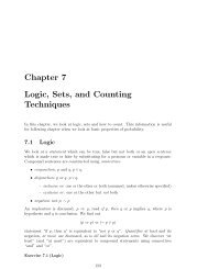
(c) Conclusion.<br />
Since p–value = 0.18 > α = 0.05,<br />
(circle one) do not reject / reject null guess: H 0 : p = 0.08.<br />
So, sample ˆp indicates population proportion p<br />
is less than / equals / is greater than 0.08: H 0 : p = 0.08.
164 Chapter <strong>10</strong>. Hypothesis Tests Regarding a Parameter (ATTENDANCE <strong>10</strong>)<br />
do not reject null<br />
p-value = 0.183<br />
reject null<br />
(critical region)<br />
α = 0.050<br />
^<br />
p = 0.08 p = 0.09<br />
z = 0 z = 0.903<br />
0<br />
null hypothesis<br />
Figure <strong>10</strong>.2(P-value for sample ˆp = 0.09, if guess p 0 = 0.08)<br />
(d) Possible mistake: Type II error.<br />
Even though hypothesis test tells us population proportion defective is<br />
equal to null H 0 : p = 0.08, we could be wrong. If we were indeed wrong,<br />
we should have picked null / alternative hypothesis H 1 : p > 0.08. Type<br />
II error is mistakenly rejecting alternative. Also, β = P(type II error).<br />
(e) Comparing hypothesis tests.<br />
P–value associated with ˆp = 0.09 (p–value = 0.183) is<br />
(choose one) smaller / larger<br />
than p–value associated with ˆp = 0.117 (p–value = 0.00).<br />
Sample proportion defective ˆp = 0.09 is<br />
(choose one) closer to / farther away from,<br />
than ˆp = 0.117, to null guess p = 0.08.<br />
It makes sense we do not reject null guess of p = 0.08 when observed<br />
proportion is ˆp = 0.09, but reject null guess when observed proportion is<br />
ˆp = 0.117.<br />
f<br />
p-value = 0.183<br />
p-value = 0.0005<br />
^<br />
p = 0.08 p = 0.09 p = 0.117<br />
z = 0 z = 0.90 z = 3.31<br />
0<br />
0<br />
null hypothesis<br />
Figure <strong>10</strong>.3(Tend to reject null for smaller p-values)<br />
If p–value is smaller than level of significance, α, reject null. If null is<br />
rejected when p–value is “really” small, less than α = 0.01, test is highly<br />
significant. If null is rejected when p–value is small, typically between<br />
^
Section 1. The Language of Hypothesis Testing (ATTENDANCE <strong>10</strong>) 165<br />
α = 0.01 and α = 0.05, test is significant. If null is not rejected, test is not<br />
significant. This is one of two approaches to hypothesis testing.<br />
(f) Comparing Type I error (α) and Type II error (β).<br />
chosen ↓ actual → null H 0 true alternative H 1 true<br />
choose null H 0 correct decision type II error, β<br />
choose alternative H 1 type I error, α correct decision: power = 1−β<br />
As α decreases, β decreases / increases because if chance of mistakenly<br />
rejecting null decreases, this necessarily means chance of mistakenly<br />
rejecting alternative increases.<br />
3. Test p, left–sided this time: defective batteries.<br />
36<br />
Of n = 600 batteries chosen at random, ths ( 36<br />
= 600 600 0.06) of them are found<br />
to be defective. Does data support possibility there is a decrease in defective<br />
batteries (from 0.08) at α = 0.05 in this case<br />
(a) Statement. Choose one.<br />
i. H 0 : p = 0.08 versus H 1 : p < 0.08<br />
ii. H 0 : p ≤ 0.08 versus H 1 : p > 0.08<br />
iii. H 0 : p = 0.08 versus H 1 : p > 0.08<br />
(b) Test.<br />
Chance ˆp = 36<br />
600 = 0.06 or less, if p 0 = 0.08, is<br />
p–value = P(ˆp ≤ 0.06) = P<br />
⎛<br />
⎝ ˆp−p 0<br />
√<br />
p0 (1−p 0 )<br />
n<br />
which equals (circle one) 0.04 / 0.06 / 0.09.<br />
⎞<br />
≤ 0.06−0.08 ⎠ ≈ P (Z ≤ −1.81) ≈<br />
√ 0.08(1−0.08)<br />
600<br />
(Options, Number of successes: 36, Number of observations: 600, Next, Null: prop. = 0.08 Alternative:<br />
< (Notice: not >!) Calculate.)<br />
Level of significance α = (choose one) 0.01 / 0.05 / 0.<strong>10</strong>.<br />
(c) Conclusion.<br />
Since p–value = 0.04 < α = 0.05,<br />
(circle one) do not reject / reject null guess: H 0 : p = 0.08.<br />
So, sample ˆp indicates population proportion p<br />
is less than / equals / is greater than 0.08: H 1 : p < 0.08.
166 Chapter <strong>10</strong>. Hypothesis Tests Regarding a Parameter (ATTENDANCE <strong>10</strong>)<br />
reject null<br />
(critical region)<br />
do not reject null<br />
f<br />
α = 0.05<br />
p-value = 0.04<br />
^<br />
p = 0.06 p = 0.08<br />
z = -1.81 z = 0<br />
0<br />
null hypothesis<br />
Figure <strong>10</strong>.4(P-value for sample ˆp = 0.06, if guess p 0 = 0.08)<br />
(d) One-sided tests.<br />
Right-sided test and left-sided tests are one-sided / two-sided tests.<br />
4. Test p, two-sided: defective batteries.<br />
36<br />
Of n = 600 batteries chosen at random, ths ( 36<br />
= 600 600 0.06) of them are found<br />
to be defective. Does data support possibility there is a change in defective<br />
batteries (from 0.08) at α = 0.05 in this case<br />
(a) Statement. Choose one.<br />
i. H 0 : p = 0.08 versus H 1 : p < 0.08<br />
ii. H 0 : p ≤ 0.08 versus H 1 : p > 0.08<br />
iii. H 0 : p = 0.08 versus H 1 : p ≠ 0.08<br />
(b) Test.<br />
Chance ˆp = 36<br />
600 = 0.06 or less, or ˆp = 0.<strong>10</strong> or more, if p 0 = 0.08, is<br />
p–value = P(ˆp ≤ 0.06)+P(ˆp ≥ 0.<strong>10</strong>)<br />
⎛<br />
⎞<br />
≈ P ⎝ ˆp−p 0<br />
√ ≤ √ 0.06−0.08 ⎠+P<br />
p0 (1−p 0 ) 0.08(1−0.08)<br />
n 600<br />
≈ P (Z ≤ −1.81)+P (Z ≥ 1.81)<br />
which equals (circle one) 0.04 / 0.07 / 0.09.<br />
⎛<br />
⎝ ˆp−p 0<br />
√<br />
p0 (1−p 0 )<br />
n<br />
⎞<br />
≥ √ 0.<strong>10</strong>−0.08 ⎠<br />
0.08(1−0.08)<br />
600<br />
(Options, Number of successes: 36, Number of observations: 600, Next, Null: prop. = 0.08 Alternative:<br />
≠ (Notice: not α = 0.05,<br />
(circle one) do not reject / reject null guess: H 0 : p = 0.08.<br />
So, sample ˆp indicates population proportion p<br />
is less than / equals / is greater than 0.08: H 0 : p = 0.08.
Section 2. Hypothesis Tests for a Population Proportion (ATTENDANCE <strong>10</strong>) 167<br />
reject null<br />
(critical region)<br />
do not reject null<br />
f<br />
reject null<br />
(critical region)<br />
p-value = 0.07/2 = 0.035<br />
α = 0.025<br />
p-value = 0.07/2 = 0.035<br />
α = 0.025<br />
^<br />
p = 0.06 p = 0.08<br />
z = -1.81 z = 0<br />
0<br />
null hypothesis<br />
^<br />
p = 0.<strong>10</strong><br />
z = 1.81<br />
0<br />
Figure <strong>10</strong>.5(Two-sided test)<br />
(d) One-sided test or two-sided test<br />
If not sure whether population proportion p above or below null guess of<br />
p 0 = 0.08, use (choose one) one-sided / two-sided test.<br />
(e) Types of tests.<br />
In this course, we are interested in<br />
right–sided test (H 0 : p = p 0 versus H 1 : p > p 0 ),<br />
left–sided test (H 0 : p = p 0 versus H 1 : p < p 0 ) and<br />
two–sided test (H 0 : p = p 0 versus H 1 : p ≠ p 0 ).<br />
However, other tests are possible; for example, (choose one or more!)<br />
i. H 0 : p < p 0 versus H 1 : p ≥ p 0<br />
ii. H 0 : p = p 0 versus H 1 : p = p 1<br />
iii. H 0 : p 0,1 ≤ p ≤ p 0,2 versus H 1 : p 0,2 ≤ p ≤ p 0,3<br />
(f) Steps in a test.<br />
Steps in any hypothesis test are (choose one or more!):<br />
i. Statement<br />
ii. Test<br />
iii. Conclusions<br />
<strong>10</strong>.2 Hypothesis Tests for a PopulationProportion<br />
Hypothesis test for p from binomial has test statistic<br />
z 0 = ˆp−p 0<br />
√<br />
p0 (1−p 0 )<br />
n<br />
where we assume a large simple random sample has been chosen, np 0 (1−p 0 ) ≥ <strong>10</strong>. If<br />
sampled from finite population, n ≤ 0.05N. We consider three approaches to testing:<br />
p-value, <strong>class</strong>ical and confidence interval. We will also discuss one-sided testing for p
168 Chapter <strong>10</strong>. Hypothesis Tests Regarding a Parameter (ATTENDANCE <strong>10</strong>)<br />
when sample size is small.<br />
Although all three approaches are mentioned, emphasis will be on p-value approach throughout course.<br />
Exercise <strong>10</strong>.2(Hypothesis Tests for a Population Proportion)<br />
1. Test p: defective batteries.<br />
Ofn = 600batterieschosenatrandom, 54 ths ( 54<br />
= 600 600 0.09) ofthemarefoundto<br />
be defective. Does data support hypotheses of an increase in defective batteries<br />
(from 0.08) at α = 0.05 in this case Solve using both p-value and <strong>class</strong>ical<br />
approaches to hypothesis testing.<br />
(a) Check assumptions.<br />
Since np 0 (1−p 0 ) = 600(0.08)(1−0.08) = 44.16 > <strong>10</strong>, assumptions<br />
have / have not been satisfied, so continue large sample test.<br />
(b) P-value approach (review).<br />
i. Statement. Choose one.<br />
A. H 0 : p = 0.08 versus H 1 : p < 0.08<br />
B. H 0 : p ≤ 0.08 versus H 1 : p > 0.08<br />
C. H 0 : p = 0.08 versus H 1 : p > 0.08<br />
ii. Test.<br />
Chance ˆp = 54<br />
600 = 0.09 or more, if p 0 = 0.08, is<br />
p–value = P(ˆp ≥ 0.09) = P<br />
⎛<br />
⎝ ˆp−p 0<br />
√<br />
p0 (1−p 0 )<br />
n<br />
which equals (circle one) 0.00 / 0.09 / 0.18.<br />
⎞<br />
≥ √ 0.09−0.08 ⎠ ≈ P (Z ≥ 0.903) ≈<br />
0.08(1−0.08)<br />
600<br />
(Stat, Proportions, Onesample, withsummary, Numberofsuccesses: 54, Numberofobservations:<br />
600, Next, Null: prop. = 0.08 Alternative: > Calculate.)<br />
Level of significance α = (choose one) 0.01 / 0.05 / 0.<strong>10</strong>.<br />
iii. Conclusion.<br />
Since p–value = 0.18 > α = 0.05,<br />
(circle one) do not reject / reject null guess: H 0 : p = 0.08.<br />
So, sample ˆp indicates population proportion p<br />
is less than / equals / is greater than 0.08: H 0 : p = 0.08.<br />
(c) Classical approach.<br />
i. Statement. Choose one.<br />
A. H 0 : p = 0.08 versus H 1 : p < 0.08<br />
B. H 0 : p ≤ 0.08 versus H 1 : p > 0.08<br />
C. H 0 : p = 0.08 versus H 1 : p > 0.08
Section 2. Hypothesis Tests for a Population Proportion (ATTENDANCE <strong>10</strong>) 169<br />
ii. Test.<br />
Test statistic<br />
z 0 = ˆp−p 0<br />
√<br />
p0 (1−p 0 )<br />
n<br />
0.90 / 1.99 / 2.18.<br />
Critical value at α = 0.05,<br />
1.28 / 1.65 / 2.58<br />
≈ 0.09−0.08 √ 0.08(1−0.08)<br />
600<br />
z α = z 0.05 ≈<br />
(Stat, Calculators, Normal, Mean: 0, Std. Dev.: 1, Prob(X ≥ ) = 0.05 Calculate.)<br />
iii. Conclusion.<br />
Since z 0 = 0.903 < z 0.05 = 1.645,<br />
(test statistic is outside critical region, so “close” to null 0.08),<br />
(circle one) do not reject / reject null guess: H 0 : p = 0.08.<br />
So, sample ˆp indicates population proportion p<br />
is less than / equals / is greater than 0.08: H 0 : p = 0.08.<br />
≈<br />
do not reject null<br />
p-value = 0.18<br />
reject null<br />
(critical region)<br />
do not reject null<br />
reject null<br />
(critical region)<br />
α = 0.05<br />
level of significance<br />
α = 0.05<br />
p = 0.08 ^p = 0.09<br />
p = 0.08 ^p = 0.09<br />
z = 0<br />
z = 0 z = 0.90 z = 1.645<br />
0 α<br />
null hypothesis null hypothesis test statistic critical value<br />
(a) p-value approach<br />
(b) <strong>class</strong>ical approach<br />
Figure <strong>10</strong>.6(P-value versus Classical Approach)<br />
(d) True / False<br />
When we do not reject null, we pick hypothesis with “equals” in it.<br />
(e) To say we do not reject null means, in this case, (circle one or more)<br />
i. disagree with claim percent defective of batteries is greater than 8%.<br />
ii. data does not support claim percent defective of batteries is greater<br />
than 8%.<br />
iii. we fail to reject percent defective of batteries equals 8%.<br />
(f) Population, Sample, Statistic, Parameter. Match columns.
170 Chapter <strong>10</strong>. Hypothesis Tests Regarding a Parameter (ATTENDANCE <strong>10</strong>)<br />
terms battery example<br />
(a) population (a) all (defective or nondefective) batteries<br />
(b) sample (b) proportion defective, of all batteries, p<br />
(c) statistic (c) 600 (defective or nondefective) batteries<br />
(d) parameter (d) proportion defective, of 600 batteries, ˆp<br />
terms (a) (b) (c) (d)<br />
example<br />
2. Test for binomial proportion, p: overweight in Indiana.<br />
An investigator wishes to know whether proportion of overweight individuals in<br />
Indiana differs from national proportion of 71% or not. A random sample of<br />
size n = 600 results in 450 ( 450<br />
600 = 0.75) who are overweight. Test at α = 0.05.<br />
(a) Check assumptions.<br />
Since np 0 (1−p 0 ) = 600(0.71)(1−0.71) = 123.54 > <strong>10</strong>, assumptions<br />
have / have not been satisfied, so continue large sample test.<br />
(b) P-value approach.<br />
i. Statement. Choose one.<br />
A. H 0 : p = 0.71 versus H 1 : p > 0.71<br />
B. H 0 : p = 0.71 versus H 1 : p < 0.71<br />
C. H 0 : p = 0.71 versus H 1 : p ≠ 0.71<br />
ii. Test.<br />
Since test statistic of ˆp = 450 = 0.75 is<br />
600<br />
z 0 = ˆp−p 0<br />
√<br />
p0 (1−p 0 )<br />
n<br />
= 0.75−0.71 √ 0.71(1−0.71)<br />
600<br />
(circle one) 1.42 / 1.93 / 2.16,<br />
chance ˆp = −0.75 or less or ˆp = 0.75 or more, if p 0 = 0.71, is<br />
p-value = P(Z ≤ −2.16)+P(Z ≥ 2.16) = 2×P(X ≥ 2.16) ≈<br />
(choose closest one) 0.031 / 0.057 / 0.075.<br />
(Stat, Proportions, One sample, with summary, Number of successes: 450, Number of observations:<br />
600, Next, Null: prop. = 0.71 Alternative: ≠ Calculate.)<br />
Level of significance α = (choose one) 0.01 / 0.05 / 0.<strong>10</strong>.<br />
iii. Conclusion.<br />
Since p–value = 0.031 < α = 0.050,<br />
(circle one) do not reject / reject null guess: H 0 : p = 0.71.<br />
In other words, sample ˆp indicates population proportion p<br />
(circle one) equals / does not equal 0.71: H 1 : p ≠ 0.71.<br />
=
Section 2. Hypothesis Tests for a Population Proportion (ATTENDANCE <strong>10</strong>) 171<br />
(c) Classical approach.<br />
i. Statement. Choose one.<br />
A. H 0 : p = 0.71 versus H 1 : p > 0.71<br />
B. H 0 : p = 0.71 versus H 1 : p < 0.71<br />
C. H 0 : p = 0.71 versus H 1 : p ≠ 0.71<br />
ii. Test.<br />
Test statistic<br />
z 0 = ˆp−p 0<br />
√<br />
p0 (1−p 0 )<br />
n<br />
0.90 / 1.99 / 2.16.<br />
Critical values at ±α = 0.05,<br />
±1.28 / ±1.65 / ±1.96<br />
±zα<br />
2 = ±z0.05<br />
2<br />
≈ 0.75−0.71 √ 0.71(1−0.71)<br />
600<br />
= ±z 0.025 ≈<br />
(Stat, Calculators, Normal, Mean: 0, Std. Dev.: 1, Prob(X ≥ ) = 0.025 Calculate.)<br />
iii. Conclusion.<br />
Since −z 0.025 = −1.96 < z 0.025 = 1.96 < z 0 = 2.16<br />
(test statistic is inside critical region, so “far away” from null 0.71),<br />
(circle one) do not reject / reject null guess: H 0 : p = 0.71.<br />
In other words, sample ˆp indicates population proportion p<br />
(circle one) equals / does not equal 0.71: H 1 : p ≠ 0.71.<br />
(d) 95% Confidence Interval (CI) for p.<br />
The 95% CI for proportion of overweight individuals, p, is<br />
(0.018,0.715) / (0.715,0.785) / (0.533,0.867).<br />
(Stat, Proportions, one sample, with summary, Number of successes: 450, Number of observations:<br />
600, choose Confidence Interval 0.95, Calculate.)<br />
Since null p 0 = 0.71 is outside CI (0.715, 0.785),<br />
(circle one) do not reject / reject null guess: H 0 : p = 0.71.<br />
In other words, sample ˆp indicates population proportion p<br />
(circle one) equals / does not equal 0.71: H 1 : p ≠ 0.71.<br />
3. Test for binomial proportion, p, small sample: conspiring Earthlings.<br />
It appears 6.5% of Earthlings are conspiring with little green mean (LGM) to<br />
take over Earth. Human versus Extraterrestrial Legion Pact (HELP) claims<br />
more than 6.5% of Earthlings are conspiring with LGM. In a random sample of<br />
<strong>10</strong>0 Earthlings, 7 ( 7<br />
= <strong>10</strong>0 0.07) are found to be conspiring with little green men<br />
(LGM). Does this data support HELP claim at α = 0.05<br />
(a) Check assumptions.<br />
Since np 0 (1−p 0 ) = <strong>10</strong>0(0.065)(1−0.065) ≈ 6.1 < <strong>10</strong>, assumptions<br />
have / have not been satisfied, so try small sample test instead.<br />
≈
172 Chapter <strong>10</strong>. Hypothesis Tests Regarding a Parameter (ATTENDANCE <strong>10</strong>)<br />
(b) Statement. Choose one.<br />
i. H 0 : p = 0.065 versus H 1 : p < 0.065<br />
ii. H 0 : p ≤ 0.065 versus H 1 : p > 0.065<br />
iii. H 0 : p = 0.065 versus H 1 : p > 0.065<br />
(c) Test.<br />
Chance ˆp = 7<br />
<strong>10</strong>0 = 0.070 or more, if p 0 = 0.065, is<br />
p–value = P(ˆp ≥ 0.07) = P(X ≥ 7) ≈<br />
(choose closest one) 0.22 / 0.32 / 0.48.<br />
(Stat, Calculators, Binomial, n: <strong>10</strong>0, p: 0.065, Prob(X ≥ 7) = Calculate.)<br />
Level of significance α = (choose one) 0.01 / 0.05 / 0.<strong>10</strong>.<br />
(d) Conclusion.<br />
Since p–value = 0.48 > α = 0.05,<br />
(circle one) do not reject / reject null guess: H 0 : p = 0.065.<br />
So, sample ˆp indicates population proportion p<br />
is less than / equals / is greater than 0.065: H 0 : p = 0.065.<br />
(e) HELP claim in this test is there are more than 6.5% conspiring Earthlings.<br />
Claim in this test, any test, for that matter, is always a statement about<br />
(circle one) null / alternative hypothesis.<br />
(f) Test constructed so if there is any doubt as to validity of HELP claim, we<br />
will fall back on not rejecting null, there are 6.5% conspiring Earthlings.<br />
Hypothesis test (always) favors (circle one) null / alternative hypothesis.<br />
(g) The p–value, in this case, is chance (choose one)<br />
i. population proportion 0.07 or more, if observed proportion 0.065.<br />
ii. observed proportion 0.07 or more, if observed proportion 0.065.<br />
iii. population proportion 0.07 or more, if population proportion 0.065.<br />
iv. observed proportion 0.07 or more, if population proportion 0.065.<br />
<strong>10</strong>.3 Hypothesis Tests for a Population Mean<br />
Hypothesis test for µ with unknown σ is a t-test with test statistic<br />
t 0 = ¯x−µ 0<br />
s/ √ n ,<br />
and used when either underlying distribution is normal with no outliers or if simple<br />
random sample size large (n ≥ 30).<br />
Exercise <strong>10</strong>.3(Mean–Population Standard Deviation Unknown)
Section 3. Hypothesis Tests for a Population Mean (ATTENDANCE <strong>10</strong>) 173<br />
1. Testing µ, right–sided: hourly wages.<br />
Average hourly wage in US is assumed to be $<strong>10</strong>.05 in 1985. Midwest big<br />
business, however, claims average hourly wage to be larger than this. A random<br />
sample of size n = 15 of midwest workers determines average hourly wage<br />
¯x = $<strong>10</strong>.83 and standard deviation in wages s = 3.25. Does data support big<br />
business’s claim at α = 0.05 Assume normality.<br />
(a) Statement. Choose one.<br />
i. H 0 : µ = $<strong>10</strong>.05 versus H 1 : µ < $<strong>10</strong>.05<br />
ii. H 0 : µ = $<strong>10</strong>.05 versus H 1 : µ ≠ $<strong>10</strong>.05<br />
iii. H 0 : µ = $<strong>10</strong>.05 versus H 1 : µ > $<strong>10</strong>.05<br />
(b) Test.<br />
Chance ¯x = <strong>10</strong>.83 or more, if µ 0 = <strong>10</strong>.05, is<br />
p–value = P( ¯X ≥ <strong>10</strong>.83) = P<br />
⎛<br />
⎝ ¯X −µ 0<br />
s √ n<br />
which equals (circle one) 0.18 / 0.20 / 0.23.<br />
⎞<br />
≥ <strong>10</strong>.83−<strong>10</strong>.05 ⎠<br />
√3.25<br />
≈ P (t ≥ 0.93) ≈<br />
15<br />
(Stat, T Statistics, with summary, Sample mean: <strong>10</strong>.83, Sample std. dev.: 3.25, Sample size: 15, Next,<br />
Null: mean = <strong>10</strong>.05, Alternative: > Calculate.)<br />
Level of significance α = (choose one) 0.01 / 0.05 / 0.<strong>10</strong>.<br />
(c) Conclusion.<br />
Since p–value = 0.18 > α = 0.05,<br />
(circle one) do not reject / reject null guess: H 0 : µ = <strong>10</strong>.05.<br />
In other words, sample ¯x indicates population average salary µ<br />
is less than / equals / is greater than <strong>10</strong>.05: H 0 : µ = <strong>10</strong>.05.<br />
(d) Match columns.<br />
terms wage example<br />
(a) population (a) all US wages<br />
(b) sample (b) wages of 15 workers<br />
(c) statistic (c) observed average wage of 15 workers<br />
(d) parameter (d) average wage of US workers, µ<br />
terms (a) (b) (c) (d)<br />
wage example<br />
2. Testing µ, right–sided: accounting program.<br />
Program director for an accounting program wishes to test, at 5%, hypothesis<br />
her students score higher than national average of 615 on national final exam.<br />
She randomly selects 11 recent graduates of two–year program and discovers<br />
¯x = 630, and s = 23. Assume underlying distribution is normal.
174 Chapter <strong>10</strong>. Hypothesis Tests Regarding a Parameter (ATTENDANCE <strong>10</strong>)<br />
(a) Statement. Choose one.<br />
i. H 0 : µ = 615 versus H 1 : µ < 615<br />
ii. H 0 : µ = 615 versus H 1 : µ ≠ 615<br />
iii. H 0 : µ = 615 versus H 1 : µ > 615<br />
(b) Test (a slightly different way).<br />
Since test statistic of ¯x = 630 is<br />
t 0 = ¯x−µ 0<br />
s/ √ n = 630−615<br />
23/ √ 11 =<br />
(circle one) 0.42 / 0.93 / 2.16,<br />
chance ¯x = 630 or more, if µ 0 = 615, is<br />
p–value = P(t ≥ 2.16) ≈ (circle one) 0.03 / 0.20 / 0.23.<br />
(Stat, T Statistics, with summary, Sample mean: 630, Sample std. dev.: 23, Sample size: 11, Next,<br />
Null: mean = 615, Alternative: > Calculate.)<br />
Level of significance α = (choose one) 0.01 / 0.05 / 0.<strong>10</strong>.<br />
(c) Conclusion.<br />
Since p–value = 0.03 < α = 0.05,<br />
(circle one) do not reject / reject null guess: H 0 : µ = 615.<br />
In other words, sample ¯x indicates program population average score µ<br />
is less than / equals / is greater than 615: H 1 : µ > 615.<br />
(d) A comment.<br />
True / False To say that this data indicates true (population) average<br />
score of her students score higher than national average also means true<br />
(population) average of all students in nation score higher on national<br />
average.<br />
(e) Related question: critical value.<br />
The critical value is t α = t 0.05 ≈ (choose one) −1.81 / 0.81 / 1.81.<br />
(Stat, Calculators, T, Mean: <strong>10</strong>, Prob(X ≥ ) = 0.05 Calculate.)<br />
3. Testing µ, right–sided, raw data: sprinkler activation time.<br />
Thirteen data values are observed in a fire-prevention study of sprinkler activation<br />
times (in seconds).<br />
27 41 22 27 23 35 30 33 24 27 28 22 24<br />
Actual average activation time is supposed to be 25 seconds. Test if it is more<br />
than this at 5%.<br />
(StatCrunch: Blank data table. Relabel var1 as time. Type 13 lengths into time column. Data, Save data,<br />
<strong>10</strong>.3 sprinkler times. OK)<br />
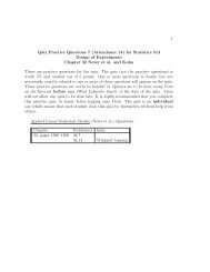
(a) Check assumptions (since n = 13 < 30): normality and outliers.
Section 3. Hypothesis Tests for a Population Mean (ATTENDANCE <strong>10</strong>) 175<br />
expected z score<br />
normal probability plot<br />
2.0<br />
boxplot of activiation times<br />
0.0<br />
-2.0<br />
20 25 30 35 40<br />
22 23.5 27 31.5 41<br />
sprinkler activiation time x<br />
Figure <strong>10</strong>.7(Normal probability plot, boxplot for times.)<br />
i. Data normal<br />
Normal probability plot indicates activation times<br />
normal / not normal because data within dotted bounds.<br />
Graphics. QQ Plot, Select Columns: time, Create Graph!<br />
ii. Outliers<br />
Boxplot indicates outliers / no outliers (but ignore it).<br />
Graphics. Boxplot, select time, Next, Use fences to identify outliers, check Draw boxes horizontally.<br />
Create Graph!<br />
(b) Statement. Choose one.<br />
i. H 0 : µ = 25 versus H 1 : µ > 25<br />
ii. H 0 : µ = 25 versus H 1 : µ < 25<br />
iii. H 0 : µ = 25 versus H 1 : µ ≠ 25<br />
(c) Test.<br />
Chance ¯x = 27.9 or more, if µ 0 = 25, is<br />
⎛<br />
p–value = P( ¯X ≥ 27.9) = P<br />
¯X<br />
⎞<br />
−µ<br />
⎝ 0<br />
√s<br />
≥ 27.9−25 ⎠<br />
5.6<br />
≈ P (t ≥ 1.88) ≈<br />
n<br />
(choose one) 0.039 / 0.043 / 0.341.<br />
(Stat, T Statistics, one sample, with data, Next, Null: mean = 25, Alternative: > Calculate.)<br />
Level of significance α = (choose one) 0.01 / 0.05 / 0.<strong>10</strong>.<br />
(d) Conclusion.<br />
Since p–value = 0.043 < α = 0.050,<br />
(circle one) do not reject / reject null guess: H 0 : µ = 25.<br />
In other words, sample ¯x indicates population average time µ<br />
is less than / equals / is greater than 25: H 0 : µ > 25.<br />
(e) Related question: unknown σ.<br />
The σ is (choose one) known / unknown in this case<br />
and is approximated by s ≈ (choose one) 5.62 / 5.73 / 5.81.<br />
(Stat, Summary Stats, Select Columns: time, Calculate.)<br />
√<br />
13
176 Chapter <strong>10</strong>. Hypothesis Tests Regarding a Parameter (ATTENDANCE <strong>10</strong>)<br />
(f) Related question: critical value.<br />
The critical value is t α = t 0.05 ≈ (choose one) −1.78 / −0.78 / 1.78.<br />
(Stat, Calculators, T, DF: 12, Prob(X ≥ ) = 0.05 Calculate.)<br />
4. Testing µ, left–sided: weight of coffee<br />
Label on a large can of Hilltop Coffee states average weight of coffee contained<br />
in all cans it produces is 3 pounds of coffee. A coffee drinker association claims<br />
average weight is less than 3 pounds of coffee, µ < 3. Suppose a random sample<br />
of 30 cans has an average weight of ¯x = 2.95 pounds and standard deviation of<br />
s = 0.18. Does data support coffee drinker association’s claim at α = 0.05<br />
(a) P-value approach.<br />
i. Statement. Choose one.<br />
A. H 0 : µ = 3 versus H 1 : µ < 3<br />
B. H 0 : µ < 3 versus H 1 : µ > 3<br />
C. H 0 : µ = 3 versus H 1 : µ ≠ 3<br />
ii. Test.<br />
Chance observed ¯x = 2.95 or less, if µ 0 = 3, is<br />
⎛<br />
p–value = P( ¯X ≤ 2.95) = P<br />
¯X<br />
⎞<br />
−µ<br />
⎝ 0<br />
√s<br />
≤ 2.95−3 ⎠<br />
√0.18<br />
≈ P (t ≤ −1.52)<br />
n 30<br />
which equals (choose one) 0.04 / 0.07 / 0.08.<br />
(Stat, T Statistics, with summary, Sample mean: 2.95, Sample std. dev.: 0.18, Sample size: 30,<br />
Next, Null: mean = 3, Alternative: < Calculate.)<br />
Level of significance α = (choose one) 0.01 / 0.05 / 0.<strong>10</strong>.<br />
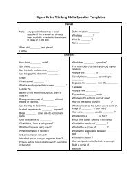
iii. Conclusion.<br />
Since p–value = 0.07 > α = 0.05,<br />
(circle one) do not reject / reject the null guess: H 0 : µ = 3.<br />
In other words, sample ¯x indicates population average weight µ<br />
(circle one) is less than / equals / is greater than 3: H 0 : µ = 3.<br />
(b) Classical approach.<br />
i. Statement. Choose one.<br />
A. H 0 : µ = 3 versus H 1 : µ < 3<br />
B. H 0 : µ < 3 versus H 1 : µ > 3<br />
C. H 0 : µ = 3 versus H 1 : µ ≠ 3<br />
ii. Test.<br />
Test statistic<br />
t 0 = ¯x−µ 0<br />
s/ √ n = 2.95−3<br />
0.18/ √ 30 ≈
Section 3. Hypothesis Tests for a Population Mean (ATTENDANCE <strong>10</strong>) 177<br />
(choose one) −1.65 / −1.52 / −1.38.<br />
Critical value at α = 0.05,<br />
t α = −t 0.05 ≈<br />
(choose one) −1.14 / −1.70 / −2.34.<br />
(Stat, Calculators, T, DF: 29, Prob(X ≤ ) = 0.05 Calculate.)<br />
iii. Conclusion.<br />
Since t 0 ≈ −1.52 > −t 0.05 ≈ −1.70,<br />
(test statistic is outside critical region, so “close” to null µ = 3),<br />
(circle one) do not reject / reject the null guess: H 0 : µ = 3.<br />
In other words, sample ¯x indicates population average weight µ<br />
(circle one) is less than / equals / is greater than 3: H 0 : µ = 3.<br />
reject null<br />
(critical region)<br />
do not reject null<br />
f<br />
reject null<br />
(critical region)<br />
do not reject null<br />
f<br />
p-value = 0.07<br />
α = 0.05<br />
α = 0.05<br />
x _ = 2.95 µ = 3<br />
t = -1.52 z = 0<br />
0<br />
null hypothesis<br />
t = -1.70<br />
α<br />
x _ = 2.95 µ = 3<br />
t = -1.52<br />
0 t = 0<br />
null hypothesis<br />
(a) p-value approach<br />
(b) <strong>class</strong>ical approach<br />
(c) Related questions.<br />
Figure <strong>10</strong>.8(Left-sided test of µ: coffee)<br />
i. “Claim” inthistest, anytest, isalwaysnull / alternativehypothesis.<br />
ii. Test always favors null / alternative hypothesis since chance of mistakenly<br />
rejecting null is so small; in this case, α = 0.05.<br />
iii. To assume null hypothesis true, means assuming (circle one)<br />
A. average weight of coffee contained in all Hilltop Coffee cans is less<br />
than 3 pounds, µ < 3.<br />
B. average weight of coffee contained in all Hilltop Coffee cans equals<br />
3 pounds, µ = 3.<br />
C. averageweight ofcoffeecontainedinarandomsampleof30Hilltop<br />
Coffee cans equals 2.95 pounds, ¯x = 2.95.<br />
iv. Match columns.
178 Chapter <strong>10</strong>. Hypothesis Tests Regarding a Parameter (ATTENDANCE <strong>10</strong>)<br />
terms coffee example<br />
(a) population (a) average weight of all cans<br />
(b) sample (b) average weight of 30 cans<br />
(c) statistic (c) weights of 30 cans<br />
(d) parameter (d) weights of all cans<br />
terms (a) (b) (c) (d)<br />
coffee example<br />
<strong>10</strong>.4 Hypothesis Tests for a Population Standard<br />
Deviation<br />
Hypothesis test for σ is a χ 2 -test with test statistic<br />
χ 2 0 = (n−1)s2 ,<br />
σ0<br />
2<br />
and used when either underlying distribution is normal with no outliers and sample<br />
is obtained using simple random sampling 1 .<br />
Exercise <strong>10</strong>.4(Hypothesis Tests for a Population Standard Deviation)<br />
1. Test for σ: car door and jamb.<br />
In a simple random sample of 28 cars, SD in gap between door and jamb is<br />
s = 0.7 mm. Test if SD is greater than 0.6 mm at α = 0.05. Assume normality<br />
with no outliers.<br />
(a) Statement. Choose one.<br />
i. H 0 : σ = 0.6 versus H 1 : σ > 0.6<br />
ii. H 0 : σ = 0.6 versus H 1 : σ < 0.6<br />
iii. H 0 : σ = 0.6 versus H 1 : σ ≠ 0.6<br />
(b) Test (p-value approach).<br />
Since degrees of freedom<br />
df = n−1 = 28−1 =<br />
(circle one) 15 / 27 / 34,<br />
chance s = 0.7 or more, if σ = 0.6, is<br />
( )<br />
(n−1)s<br />
2<br />
p–value = P(s ≥ 0.7) = P ≥ (28−1)(0.72 )<br />
≈ P ( χ 2 ≥ 36.75 ) ≈<br />
σ 2 0.6 2<br />
1 This test is used not only for SD σ but also variance σ 2 . CI is sensitive to non-normal data<br />
which is not always fixed by large sample size.
Section4. HypothesisTestsforaPopulationStandardDeviation(ATTENDANCE<strong>10</strong>)179<br />
(circle one) 0.01 / 0.05 / 0.<strong>10</strong>.<br />
(Stat, Variance, with summary, Sample variance: 0.49, Sample size: 28, Next, Null: mean = 0.36,<br />
Alternative: > Calculate. Notice, SDs must be squared to variances to use StatCrunch.)<br />
Level of significance α = (choose one) 0.01 / 0.05 / 0.<strong>10</strong>.<br />
(c) Conclusion.<br />
Since p–value = 0.<strong>10</strong> > α = 0.05,<br />
(circle one) do not reject / reject null guess: H 0 : σ = 0.6.<br />
So, sample s indicates population SD σ<br />
is less than / equals / is greater than 0.6: H 0 : σ = 0.6.<br />
f<br />
do not reject null<br />
reject null<br />
(critical region)<br />
p-value = 0.<strong>10</strong><br />
α = 0.05<br />
0 <strong>10</strong> 20 30 40 50<br />
s = 0.7<br />
χ 2 = 36.75<br />
0<br />
Figure <strong>10</strong>.9(Right-sided χ 2 test of σ)<br />
(d) Population, parameter, sample and statistic. Match columns.<br />
terms jamb example<br />
(a) population (a) SD in jamb–door distance, of 28 cars, s<br />
(b) sample (b) SD in jamb–door distance, of all cars, σ<br />
(c) statistic (c) jamb–door distances, of all cars<br />
(d) parameter (d) jamb–door distances, of 28 cars<br />
terms (a) (b) (c) (d)<br />
jamb example<br />
2. Inference for variance: machine parts.<br />
In a random sample of 18 machine parts, SD in lengths is s = 12 mm. Test if<br />
SD is less than 13 mm at α = 0.05.<br />
(a) Statement. The statement of the test is (circle one)<br />
i. H 0 : σ = 13 versus H 1 : σ > 13<br />
ii. H 0 : σ = 13 versus H 1 : σ < 13<br />
iii. H 0 : σ = 13 versus H 1 : σ ≠ 13
180 Chapter <strong>10</strong>. Hypothesis Tests Regarding a Parameter (ATTENDANCE <strong>10</strong>)<br />
(b) Test (<strong>class</strong>ical approach).<br />
Test statistic of s = 12 is<br />
χ 2 0 = (n−1)s2<br />
σ 2 0<br />
= (18−1)(12)2<br />
13 2 =<br />
(circle one) 14.48 / 60.41 / 82.47.<br />
(Stat, Variance, with summary, Sample variance: 144, Sample size: 18, Next, Null: mean = 169,<br />
Alternative: < Calculate. Again notice SDs must be squared to variances to use StatCrunch.)<br />
with degrees of freedom<br />
(circle one) 15 / 17 / 34 df,<br />
Lower critical value at α = 0.05,<br />
(choose one) 7.67 / 8.67 / 9.67.<br />
n −1 = 18−1 =<br />
χ 2 1−α = χ2 0.95 ≈<br />
(Stat, Calculators, Chi-square, DF: 17, Prob(X ≥ ) = 0.95 Calculate.)<br />
(c) Conclusion.<br />
Since χ 2 0 ≈ 14.45 > χ 2 0.95 ≈ 8.67,<br />
(test statistic is outside critical region, so “close” to null σ = 13),<br />
(circle one) do not reject / reject null guess: H 0 : σ = 13.<br />
In other words, sample s indicates population SD σ<br />
(circle one) is less than / equals / is greater than 13: H 0 : σ = 13.<br />
f<br />
reject null<br />
(critical region)<br />
do not reject null<br />
α = 0.05<br />
0 5 <strong>10</strong> 15 20 25<br />
χ 2= 8.67<br />
α<br />
s = 12<br />
χ 2 = 14.45<br />
0<br />
Figure <strong>10</strong>.<strong>10</strong>(Left-sided χ 2 test of σ)<br />
<strong>10</strong>.5 Putting It Together: Which Method Do I<br />
Use<br />
The following table summaries all of the hypothesis tests given in this chapter and<br />
under what circumstances to calculate any one of these hypothesis tests; other hy-
Section7. TheProbabilityofaTypeIIErrorandthePoweroftheTest(ATTENDANCE<strong>10</strong>)181<br />
pothesis tests are given in later chapters. This table has also been used in earlier<br />
chapters to summarize confidence intervals.<br />
HYPOTHESIS mean variance proportion<br />
TESTS µ σ 2 p<br />
one z 0 = ¯x−µ 0<br />
σ/ √ n<br />
χ 2 0 = (n−1)s2<br />
σ 2 0<br />
ˆp−p<br />
large: z 0 = √ 0<br />
p0 (1−p 0 )<br />
n<br />
small: use binomial<br />
sample two chapter 11 chapter 11 chapter 11<br />
multiple chapter 13 not covered chapter 12<br />
<strong>10</strong>.6 The Probability of a Type II Error and the<br />
Power of the Test<br />
Not covered.