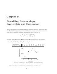
Homework 3 (Attendance 5) for Statistics 512 Applied Regression ...
Homework 3 (Attendance 5) for Statistics 512 Applied Regression ...
Homework 3 (Attendance 5) for Statistics 512 Applied Regression ...

You also want an ePaper? Increase the reach of your titles
YUMPU automatically turns print PDFs into web optimized ePapers that Google loves.
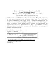
<strong>Homework</strong> 3 (<strong>Attendance</strong> 5) <strong>for</strong> <strong>Statistics</strong> <strong>512</strong><br />
<strong>Applied</strong> <strong>Regression</strong> Analysis<br />
Material Covered: Chapter 6 Neter et al. and Kuhn<br />
By: Friday, 3rd October, Fall 2003<br />
This homework is worth 5% and marked out of 5 points. <strong>Homework</strong> assignments<br />
are to be handed in using Vista on the Internet be<strong>for</strong>e 4am. Vista will not allow<br />
any homework assignment to be handed in late. It is highly recommended that you<br />
complete the homework, by hand, be<strong>for</strong>e logging onto Vista; use Vista simply to<br />
submit your answers. Submit as many times as you want be<strong>for</strong>e the deadline and<br />
receive the highest score of all the submissions. This is an individual homework<br />
and so each student submits their own homework, although they are encouraged to<br />
cooperate with other students.<br />
1. <strong>Applied</strong> Linear Statistical Models<br />
(Neter et al.) Questions.<br />
Chapter Problem(s) hints<br />
6, pages 252–257 6.9, 6.10, 6.11, 6.12, 6.13, 6.14 Chemical shipment<br />
6.18, 6.19, 6.20, 6.21 Mathematicians’ salaries
(6.9) chemical shipment, hw3-6-9-chem-diagnos<br />
*HOMEWORK 3, 6-9, PAGES 252-257;<br />
DATA CHEMICAL;<br />
INPUT Y X1 X2 TIME;<br />
DATALINES;<br />
58 7 5.11 1<br />
152 18 16.72 2<br />
41 5 3.2 3<br />
93 14 7.03 4<br />
101 11 10.98 5<br />
38 5 4.04 6<br />
203 23 22.07 7<br />
78 9 7.03 8<br />
117 16 10.62 9<br />
44 5 4.76 10<br />
121 17 11.02 11<br />
112 12 9.51 12<br />
50 6 3.79 13<br />
82 12 6.45 14<br />
48 8 4.6 15<br />
127 15 13.86 16<br />
140 17 13.03 17<br />
155 21 15.21 18<br />
39 6 3.64 19<br />
90 11 9.57 20<br />
;<br />
*6.9(A) STEM AND LEAF OF X1 AND X2;<br />
PROC UNIVARIATE DATA=CHEMICAL PLOT;<br />
TITLE1 '6.9(A) STEM AND LEAF OF NUMBER OF DRUMS, X1';<br />
TITLE2 'AND OF WEIGHT OF SHIPMENTS, X2';<br />
VAR X1 X2;<br />
RUN;<br />
*6.9(B) TIMEPLOTS OF HANDLING MINUTES;<br />
SYMBOL1 V=STAR C=BLACK;<br />
PROC GPLOT DATA=CHEMICAL;<br />
TITLE1 '6.9(B-1) TIMEPLOT OF NUMBER OF DRUMS, X1';<br />
PLOT X1*TIME;<br />
RUN;<br />
SYMBOL1 V=STAR C=BLACK;<br />
PROC GPLOT DATA=CHEMICAL;<br />
TITLE1 '6.9(B-2) TIMEPLOT OF WEIGHT OF SHIPMENTS, X2';<br />
PLOT X2*TIME;<br />
RUN;<br />
*6.9(C) SCATTERPLOT MATRICES AND CORRELATION;<br />
SYMBOL1 V=STAR C=BLACK;<br />
PROC GPLOT DATA=CHEMICAL;<br />
TITLE1 '6.9(C-1) HANDING TIME VERSUS NUMBER OF DRUMS, Y VS X1';<br />
PLOT Y*X1;<br />
RUN;<br />
SYMBOL1 V=STAR C=BLACK;<br />
PROC GPLOT DATA=CHEMICAL;<br />
TITLE1 '6.9(C-2) HANDING TIME VERSUS NUMBER OF DRUMS, Y VS X2';<br />
PLOT Y*X2;<br />
RUN;<br />
SYMBOL1 V=STAR C=BLACK;<br />
PROC GPLOT DATA=CHEMICAL;<br />
TITLE1 '6.9(C-3) HANDING TIME VERSUS NUMBER OF DRUMS, X1 VS X2';<br />
PLOT X1*X2;<br />
RUN;<br />
PROC CORR DATA=CHEMICAL;<br />
TITLE '6.9(C-4) CORRELATION Y, X1 AND X2';<br />
VAR Y X1 X2;<br />
RUN;<br />
QUIT;<br />
(a) Stem–and–leaf plots.<br />
Look <strong>for</strong> outliers.<br />
(b) Time Plots.<br />
Any patterns
(c) Scatter plots and correlation matrix<br />
It would be “good” that Y is strongly linearly related to both X 1 and X 2 ,<br />
but it would be “bad” that X 1 and X 2 are strongly linearly related to one<br />
another.
(6.10) chemical shipment again, hw3-6-10-chem-residual<br />
*HOMEWORK 3, 6-10, PAGES 252-257;<br />
DATA CHEMICAL;<br />
INPUT Y X1 X2 TIME;<br />
X1X2 = X1*X2;<br />
DATALINES;<br />
58 7 5.11 1<br />
152 18 16.72 2<br />
41 5 3.2 3<br />
93 14 7.03 4<br />
101 11 10.98 5<br />
38 5 4.04 6<br />
203 23 22.07 7<br />
78 9 7.03 8<br />
117 16 10.62 9<br />
44 5 4.76 10<br />
121 17 11.02 11<br />
112 12 9.51 12<br />
50 6 3.79 13<br />
82 12 6.45 14<br />
48 8 4.6 15<br />
127 15 13.86 16<br />
140 17 13.03 17<br />
155 21 15.21 18<br />
39 6 3.64 19<br />
90 11 9.57 20<br />
;<br />
*6.10(A) REGRESSION;<br />
PROC REG DATA=CHEMICAL OUTEST=EST;<br />
TITLE1 '6.10(A) REGRESSION OF Y VS X1 AND X2';<br />
MODEL Y = X1 X2;<br />
OUTPUT OUT=OUTPLOT PREDICTED=PRED RESIDUAL=RESID;<br />
RUN;<br />
*6.10(B) BOXPLOT OF RESIDUALS;<br />
PROC UNIVARIATE DATA=OUTPLOT PLOT;<br />
TITLE1 '6.10(B) BOXPLOT OF RESIDUALS';<br />
VAR RESID;<br />
RUN;<br />
*6.10(C) RESIDUALS VS PREDICTED, X1, X2 AND X1X2;<br />
SYMBOL1 V=STAR C=BLACK;<br />
PROC GPLOT DATA=OUTPLOT;<br />
TITLE '6.10(C-1) RESIDUALS VS PREDICTED';<br />
PLOT RESID*PRED;<br />
RUN;<br />
SYMBOL1 V=STAR C=BLACK;<br />
PROC GPLOT DATA=OUTPLOT;<br />
TITLE '6.10(C-2) RESIDUALS VS X1';<br />
PLOT RESID*X1;<br />
RUN;<br />
SYMBOL1 V=STAR C=BLACK;<br />
PROC GPLOT DATA=OUTPLOT;<br />
TITLE '6.10(C-3) RESIDUALS VS X2';<br />
PLOT RESID*X2;<br />
RUN;<br />
SYMBOL1 V=STAR C=BLACK;<br />
PROC GPLOT DATA=OUTPLOT;<br />
TITLE '6.10(C-4) RESIDUALS VS X1X2';<br />
PLOT RESID*X1X2;<br />
RUN;<br />
*6.10(C) NORMAL PROBABILITY PLOT;<br />
* RESIDUALS VS EXPECTED RESIDUALS;<br />
PROC SORT DATA=OUTPLOT;<br />
BY RESID;<br />
RUN;<br />
DATA OUTPLOT;<br />
SET OUTPLOT NOBS=NOBS;<br />
QUANTILE = PROBIT( (_N_- (3/8)) / (NOBS + (1/4)) );<br />
RUN;<br />
DATA OUTPLOT2;<br />
IF _N_ = 1 THEN SET EST;<br />
SET OUTPLOT;<br />
EXPRESIDUAL = _RMSE_*QUANTILE;<br />
RUN;<br />
PROC GPLOT DATA=OUTPLOT2;<br />
TITLE '6.10(C-5) NORMAL PROBABILITY PLOT';<br />
PLOT RESID*EXPRESIDUAL;<br />
RUN;<br />
*6.10(D) TIMEPLOT OF RESIDUALS;<br />
SYMBOL1 V=STAR C=BLACK;<br />
PROC GPLOT DATA=OUTPLOT;<br />
TITLE1 '6.10(D) TIMEPLOT OF RESIDUALS';<br />
PLOT RESID*TIME;<br />
RUN;<br />
*6.10(E) LEVENE TEST OF RESIDUALS;<br />
DATA NEWCHEMICAL;<br />
SET OUTPLOT;<br />
IF PRED < 92 THEN LEVENEGROUP = 'A';<br />
IF PRED GE 92 THEN LEVENEGROUP = 'B';<br />
RUN;<br />
PROC GLM DATA=NEWCHEMICAL ALPHA=0.01;<br />
TITLE '6.10(E) (UNMODIFIED) LEVENE TEST';<br />
TITLE1 'OF HOMOGENEITY OF VARIANCE OF RESIDUALS';<br />
CLASS LEVENEGROUP;<br />
MODEL RESID = LEVENEGROUP;<br />
MEANS LEVENEGROUP / HOVTEST = LEVENE (TYPE=ABS);<br />
RUN;<br />
QUIT;
(a) Estimated regression function.<br />
(b) Box plot of the residuals.<br />
Look <strong>for</strong> outliers.<br />
(c) Residual plots.<br />
It is “good” if there is no pattern or outliers in residual plots.<br />
(d) Residuals versus time plot.<br />
(e) Levene Test<br />
1. Statement.<br />
The statement of the test is (check none, one or more):<br />
(i) H 0 : error variance constant versus H 1 : ρ > 1.<br />
(ii) H 0 : error variance constant versus H 1 : not constant<br />
(iii) H 0 : error variance constant versus H 1 : ρ ≠ 1.<br />
2. Test.<br />
From SAS, the p–value is (choose one) 0.446 / 0.8278 / 0.989<br />
The level of significance is (circle one) 0.01 / 0.05 / .10<br />
3. Conclusion.<br />
Since the p–value is smaller / larger than the level of significance we<br />
(circle one) accept / reject the null hypothesis that the error variance<br />
is constant.
(6.11) chemical shipment again, hw3-6-11-chem-regress<br />
*HOMEWORK 3, 6-11, PAGES 252-257;<br />
DATA CHEMICAL;<br />
INPUT Y X1 X2 TIME;<br />
DATALINES;<br />
58 7 5.11 1<br />
152 18 16.72 2<br />
41 5 3.2 3<br />
93 14 7.03 4<br />
101 11 10.98 5<br />
38 5 4.04 6<br />
203 23 22.07 7<br />
78 9 7.03 8<br />
117 16 10.62 9<br />
44 5 4.76 10<br />
121 17 11.02 11<br />
112 12 9.51 12<br />
50 6 3.79 13<br />
82 12 6.45 14<br />
48 8 4.6 15<br />
127 15 13.86 16<br />
140 17 13.03 17<br />
155 21 15.21 18<br />
39 6 3.64 19<br />
90 11 9.57 20<br />
;<br />
*6.11 REGRESSION;<br />
PROC REG DATA=CHEMICAL;<br />
TITLE1 '6.11 REGRESSION OF Y VS X1 AND X2';<br />
MODEL Y = X1 X2;<br />
RUN;<br />
QUIT;<br />
Source Sum Of Squares Degrees of Freedom Mean Squares<br />
<strong>Regression</strong> 40,496.48 p − 1 = 3 − 1 = 2 20,248.24<br />
Error 536.47 n − p = 20 − 3 = 17 31.56<br />
Total 41,032.95 n − 1 = 20 − 1 = 19<br />
(a) Test of regression relation at α = 0.05.<br />
1. Statement.<br />
The statement of the test is (check none, one or more):<br />
(i) H 0 : β 1 = β 2 = 0 versus H 1 : β 1 = β 2 > 0.<br />
(ii) H 0 : β 1 = β 2 = 0 versus H 1 : β 1 = β 2 < 0.<br />
(iii) H 0 : β 1 = β 2 = 0 versus H 1 : not all β i is zero.<br />
2. Test.<br />
From SAS, the p–value is (choose one) 0 / 0.0827 / 0.098<br />
The level of significance is (circle one) 0.01 / 0.05 / .10<br />
3. Conclusion.<br />
Since the p–value is smaller / larger than the level of significance we<br />
(circle one) accept / reject the null hypothesis that β 1 = β 2 = 0.
(b) Bonferroni Confidence Intervals.<br />
From TI–83 (INVT 18 ENTER 0.975 ENTER)<br />
B = t(1 − α/2g; n − 2) = t(1 − 0.05/2(2); 20 − 2) = t(0.9875; 18) = 2.458<br />
From SAS,<br />
1. Bonferroni CI <strong>for</strong> β 1 :<br />
b 1 = 3.7681 and s{b 1 } = 0.614,<br />
b 1 ± Bs{b 1 } = 3.7681 ± 2.458(0.614) =<br />
2. Bonferroni CI <strong>for</strong> β 2 :<br />
b 2 = 5.0796 and s{b 2 } = 0.666<br />
b 2 ± Bs{b 2 } = 5.0796 ± 2.458(0.666) =<br />
(c) Correlation Coefficient.<br />
R 2 = SSR = 40,496.48 ≈ 0.987<br />
SSTO 41,032.95<br />
R 2 is also given directly on the SAS output
(6.12) chemical shipment again, hw3-6-12-chem-respCI<br />
*HOMEWORK 3, 6-12, PAGES 252-257;<br />
DATA CHEMICALX;<br />
INPUT Y X1 X2 TIME;<br />
DATALINES;<br />
58 7 5.11 1<br />
152 18 16.72 2<br />
41 5 3.2 3<br />
93 14 7.03 4<br />
101 11 10.98 5<br />
38 5 4.04 6<br />
203 23 22.07 7<br />
78 9 7.03 8<br />
117 16 10.62 9<br />
44 5 4.76 10<br />
121 17 11.02 11<br />
112 12 9.51 12<br />
50 6 3.79 13<br />
82 12 6.45 14<br />
48 8 4.6 15<br />
127 15 13.86 16<br />
140 17 13.03 17<br />
155 21 15.21 18<br />
39 6 3.64 19<br />
90 11 9.57 20<br />
. 5 3.20 21<br />
. 6 4.80 22<br />
. 10 7.00 23<br />
. 14 10.00 24<br />
. 20 18.00 25<br />
;<br />
DATA CHEMICAL X;<br />
SET CHEMICALX;<br />
IF READ NE . THEN OUTPUT CHEMICAL;<br />
ELSE OUTPUT X;<br />
RUN;<br />
PROC REG DATA=CHEMICAL ALPHA=0.05 NOPRINT;<br />
TITLE '6.12(A) BONFERRONI AND WH JOINT CIs FOR MEAN';<br />
MODEL Y = X1 X2;<br />
OUTPUT OUT=OUTPLOT PREDICTED=PRED RESIDUAL=RESID;<br />
RUN;<br />
PROC REG DATA=CHEMICALX;<br />
MODEL Y = X1 X2;<br />
OUTPUT OUT=PRED_DS(WHERE=(Y =.)) P=PHAT STDP=STDP;<br />
RUN;<br />
PROC PRINT DATA=PRED_DS;<br />
RUN;<br />
PROC PLOT DATA=CHEMICALX;<br />
TITLE '6.12(B) RANGE OF X1 AND X2';<br />
PLOT X1*X2=Y;<br />
RUN;<br />
PROC G3D DATA=CHEMICALX;<br />
SCATTER X1*X2=Y;<br />
RUN;<br />
QUIT;<br />
(a) Family CIs For Different Responses.<br />
At α = 0.05, and g = 5 (five simultaneous intervals),<br />
from TI–83, √<br />
√<br />
W = pF (1 − α; p, n − p) = 3F (1 − 0.05; 3, 20 − 3) = 3.098<br />
(INVF 3 ENTER 17 ENTER 0.95 ENTER,<br />
then multiply by 3 and find the square root)<br />
B = t(1 − α/2g; n − p) = t(1 − 0.05/2(5); 20 − 3) = t(0.995; 17) = 2.898<br />
(INVT 17 ENTER 0.995 ENTER)<br />
Since W = 3.098 > B = 2.898, use <br />
From SAS,<br />
1. X h1 = 5, X h2 = 3.20:
Ŷ h = 38.4195 and s{Ŷh} = 2.0332<br />
Ŷ h ± Bs{Ŷh} = 38.4195 ± 2.898(2.0332) =<br />
2. X h1 = 6, X h2 = 4.80:<br />
Ŷ h = 50.3150 and s{Ŷh} = 1.9192<br />
Ŷ h ± Bs{Ŷh} = 50.3150 ± 2.898(1.9192) =<br />
3. X h1 = 10, X h2 = 7.00:<br />
Ŷ h = 76.5625 and s{Ŷh} = 1.3701<br />
Ŷ h ± Bs{Ŷh} = 76.5625 ± 2.898(1.3701) =<br />
4. X h1 = 14, X h2 = 10.00:<br />
Ŷ h = 106.8737 and s{Ŷh} = 1.4761<br />
Ŷ h ± Bs{Ŷh} = 106.8737 ± 2.898(1.4761) =<br />
5. X h1 = 20, X h2 = 18.00:<br />
Ŷ h = 170.1191 and s{Ŷh} = 2.6096<br />
Ŷ h ± Bs{Ŷh} = 170.1191 ± 2.898(2.6096) =<br />
(b) Plot X i1 versus X i2 .<br />
The point (X 1 , X 2 ) = (20, 5) is clearly where in the the scatter of points<br />
The point (X 1 , X 2 ) = (20, 19) is clearly where in the the scatter of points
(6.13) chemical shipment again, hw3-6-13-chem-respPI<br />
*HOMEWORK 3, 6-13, PAGES 252-257;<br />
DATA CHEMICAL;<br />
INPUT Y X1 X2 TIME;<br />
DATALINES;<br />
58 7 5.11 1<br />
152 18 16.72 2<br />
41 5 3.2 3<br />
93 14 7.03 4<br />
101 11 10.98 5<br />
38 5 4.04 6<br />
203 23 22.07 7<br />
78 9 7.03 8<br />
117 16 10.62 9<br />
44 5 4.76 10<br />
121 17 11.02 11<br />
112 12 9.51 12<br />
50 6 3.79 13<br />
82 12 6.45 14<br />
48 8 4.6 15<br />
127 15 13.86 16<br />
140 17 13.03 17<br />
155 21 15.21 18<br />
39 6 3.64 19<br />
90 11 9.57 20<br />
;<br />
PROC IML;<br />
USE CHEMICAL;<br />
READ ALL VAR {'X1'} INTO X1;<br />
READ ALL VAR {'X2'} INTO X2;<br />
READ ALL VAR {'Y'} INTO Y;<br />
N = NROW(X1);<br />
M = NCOL(Y);<br />
J = J(N,N,1);<br />
X = J(N,1,1)||X1||X2;<br />
B = INV(X`*X)*X`*Y;<br />
H = X*INV(X`*X)*X`;<br />
SSE = Y`*(I(N) - H)*Y;<br />
DFE = N - 3;<br />
MSE = SSE/DFE;<br />
XH = { 1 1 1 1,<br />
9 12 15 18,<br />
7.20 9.00 12.50 16.50};<br />
YHAT = XH`*B;<br />
*SQRT WORKS BECAUSE NO NEGATIVES!;<br />
SPRED = SQRT(MSE*(1 + XH`*INV(X`*X)*XH));<br />
PRINT YHAT;<br />
PRINT S2PRED;<br />
PRINT SPRED;<br />
RUN;<br />
QUIT;<br />
At α = 0.05, g = 4 (four simultaneous intervals)<br />
and p = 3 (three parameters, β 0 ,β 1 , β 2 ),<br />
from√TI–83,<br />
√<br />
S = gF (1 − α; g, n − p) = 4F (1 − 0.05; 4, 20 − 3) = 3.441<br />
(INVF 4 ENTER 17 ENTER 0.95 ENTER,<br />
then multiply by 4 and find the square root)<br />
B = t(1 − α/2g; n − p) = t(1 − 0.05/2(4); 20 − 3) = t(0.99375; 17) = 2.793<br />
(INVT 17 ENTER 0.995 ENTER)<br />
Since S = 3.441 > B = 2.793, use B because the Bonferroni gives narrower<br />
(more efficient) CIs than the Scheffe CIs.<br />
From SAS,
1. X h1 = 9, X h2 = 7.20:<br />
Ŷ h = 73.8103 and s{pred} = 5.8076<br />
Ŷ h ± Bs{Ŷh} = 73.8103 ± 2.793(5.8076) =<br />
2. X h1 = 12, X h2 = 9.00:<br />
Ŷ h = 94.2579 and s{pred} = 5.7578<br />
Ŷ h ± Bs{Ŷh} = 94.2579 ± 2.793(5.7578) =<br />
3. X h1 = 15, X h2 = 12.50:<br />
Ŷ h = 123.3408 and s{pred} = 5.8217<br />
Ŷ h ± Bs{Ŷh} = 123.3408 ± 2.793(5.8217) =<br />
4. X h1 = 18, X h2 = 16.50:<br />
Ŷ h = 154.9635 and s{pred} = 6.1013<br />
Ŷ h ± Bs{Ŷh} = 154.9635 ± 2.793(6.1013) =
(6.14) chemical shipment again, hw3-6-14-chem-respPmean<br />
*HOMEWORK 3, 6-14, PAGES 252-257;<br />
DATA CHEMICAL;<br />
INPUT Y X1 X2 TIME;<br />
DATALINES;<br />
58 7 5.11 1<br />
152 18 16.72 2<br />
41 5 3.2 3<br />
93 14 7.03 4<br />
101 11 10.98 5<br />
38 5 4.04 6<br />
203 23 22.07 7<br />
78 9 7.03 8<br />
117 16 10.62 9<br />
44 5 4.76 10<br />
121 17 11.02 11<br />
112 12 9.51 12<br />
50 6 3.79 13<br />
82 12 6.45 14<br />
48 8 4.6 15<br />
127 15 13.86 16<br />
140 17 13.03 17<br />
155 21 15.21 18<br />
39 6 3.64 19<br />
90 11 9.57 20<br />
;<br />
PROC IML;<br />
USE CHEMICAL;<br />
READ ALL VAR {'X1'} INTO X1;<br />
READ ALL VAR {'X2'} INTO X2;<br />
READ ALL VAR {'Y'} INTO Y;<br />
N = NROW(X1);<br />
M = NCOL(Y);<br />
J = J(N,N,1);<br />
X = J(N,1,1)||X1||X2;<br />
B = INV(X`*X)*X`*Y;<br />
H = X*INV(X`*X)*X`;<br />
SSE = Y`*(I(N) - H)*Y;<br />
DFE = N - 3;<br />
MSE = SSE/DFE;<br />
XH = { 1 1 1,<br />
7 7 7,<br />
6 6 6};<br />
YHAT = XH`*B;<br />
*SQRT WORKS BECAUSE NO NEGATIVES!;<br />
SPRED = SQRT(MSE*(1/3 + XH`*INV(X`*X)*XH));<br />
PRINT YHAT;<br />
PRINT SPRED;<br />
RUN;<br />
QUIT;<br />
(a) Mean of New Observations CI.<br />
At α = 0.05, p = 3 (three parameters, β 0 , β 1 , β 2 ),<br />
and m = 3 (mean of three new observations)<br />
from TI–83,<br />
B = t(1 − α/2; n − p) = t(1 − 0.05/2; 20 − 3) = t(0.975; 17) = 2.110<br />
(INVT 17 ENTER 0.975 ENTER)<br />
X h1 = 7, X h2 = 6:<br />
Ŷ h = 60.1786 and s{predmean} = 3.7281<br />
Ŷ h ± Bs{Ŷh} = 60.1786 ± 2.110(3.7281) =<br />
(b) A CI <strong>for</strong> the total handling time, then, would be<br />
3 × (52.30, 68.04) =
(6.18) Mathematicians’ salaries, hw3-6-18-math-diagnos<br />
*HOMEWORK 3, 6-18, PAGES 252-257;<br />
DATA MATH;<br />
INPUT Y X1 X2 X3;<br />
X1X2 = X1*X2;<br />
X1X3 = X1*X3;<br />
X2X3 = X2*X3;<br />
DATALINES;<br />
33.2 3.5 9 6.1<br />
40.3 5.3 20 6.4<br />
38.7 5.1 18 7.4<br />
46.8 5.8 33 6.7<br />
41.4 4.2 31 7.5<br />
37.5 6 13 5.9<br />
39 6.8 25 6<br />
40.7 5.5 30 4<br />
30.1 3.1 5 5.8<br />
52.9 7.2 47 8.3<br />
38.2 4.5 25 5<br />
31.8 4.9 11 6.4<br />
43.3 8 23 7.6<br />
44.1 6.5 35 7<br />
42.8 6.6 39 5<br />
33.6 3.7 21 4.4<br />
34.2 6.2 7 5.5<br />
48 7 40 7<br />
38 4 35 6<br />
35.9 4.5 23 3.5<br />
40.4 5.9 33 4.9<br />
36.8 5.6 27 4.3<br />
45.2 4.8 34 8<br />
35.1 3.9 15 5<br />
;<br />
*6.18(A) STEM AND LEAF OF X1, X2 AND X3;<br />
PROC UNIVARIATE DATA=MATH PLOT;<br />
TITLE1 '6.18(A) STEM AND LEAF OF WORK QUALITY, X1';<br />
TITLE2 'AND OF YEARS OF EXPERIENCE, X2';<br />
TITLE3 'AND OF PUBLICATION SUCCESS, X3';<br />
VAR X1 X2 X3;<br />
RUN;<br />
*6.18(B) SCATTERPLOT MATRICES AND CORRELATION;<br />
SYMBOL1 V=STAR C=BLACK;<br />
PROC GPLOT DATA=MATH;<br />
TITLE '6.18(B) SCATTERPLOT MATRICES';<br />
PLOT Y*X1;<br />
PLOT Y*X2;<br />
PLOT Y*X3;<br />
PLOT X1*X2;<br />
PLOT X1*X3;<br />
PLOT X2*X3;<br />
RUN;<br />
PROC CORR DATA=MATH;<br />
TITLE '6.18(C-4) CORRELATION Y, X1, X2 AND X3';<br />
VAR Y X1 X2 X3;<br />
RUN;<br />
*6.18(C) REGRESSION;<br />
PROC REG DATA=MATH OUTEST=EST;<br />
TITLE1 '6.18(C) REGRESSION OF Y VS X1, X2 AND X3';<br />
MODEL Y = X1 X2 X3;<br />
OUTPUT OUT=OUTPLOT PREDICTED=PRED RESIDUAL=RESID;<br />
RUN;<br />
*6.18(D) BOXPLOT OF RESIDUALS;<br />
PROC UNIVARIATE DATA=OUTPLOT PLOT;<br />
TITLE1 '6.18(D) BOXPLOT OF RESIDUALS';<br />
VAR RESID;<br />
RUN;<br />
*6.18(E) RESIDUALS VS PREDICTED, X1, X2, X3 AND INTERACTIONS;<br />
SYMBOL1 V=STAR C=BLACK;<br />
PROC GPLOT DATA=OUTPLOT;<br />
TITLE '6.18(E-1) RESIDUALS VS VARIOUS';<br />
PLOT RESID*PRED;<br />
PLOT RESID*X1;<br />
PLOT RESID*X2;<br />
PLOT RESID*X3;<br />
PLOT RESID*X1X2;<br />
PLOT RESID*X1X3;<br />
PLOT RESID*X2X3;<br />
RUN;<br />
PROC SORT DATA=OUTPLOT;<br />
BY RESID;<br />
RUN;<br />
DATA OUTPLOT;<br />
SET OUTPLOT NOBS=NOBS;<br />
QUANTILE = PROBIT( (_N_- (3/8)) / (NOBS + (1/4)) );<br />
RUN;<br />
DATA OUTPLOT2;<br />
IF _N_ = 1 THEN SET EST;<br />
SET OUTPLOT;<br />
EXPRESIDUAL = _RMSE_*QUANTILE;<br />
RUN;<br />
PROC GPLOT DATA=OUTPLOT2;<br />
TITLE '6.18(E-2) NORMAL PROBABILITY PLOT';<br />
PLOT RESID*EXPRESIDUAL;<br />
RUN;<br />
*6.10(F) LEVENE TEST OF RESIDUALS;<br />
DATA NEWMATH;<br />
SET OUTPLOT;<br />
IF PRED < 38.75 THEN LEVENEGROUP = 'A';<br />
IF PRED GE 38.75 THEN LEVENEGROUP = 'B';<br />
RUN;<br />
PROC GLM DATA=NEWMATH ALPHA=0.05;<br />
TITLE '6.18(F) (UNMODIFIED) LEVENE TEST';<br />
TITLE1 'OF HOMOGENEITY OF VARIANCE OF RESIDUALS';<br />
CLASS LEVENEGROUP;<br />
MODEL RESID = LEVENEGROUP;<br />
MEANS LEVENEGROUP / HOVTEST = LEVENE (TYPE=ABS);<br />
RUN;<br />
QUIT;
(a) Stem and Leaf Plots.<br />
(b) Scatterplots and Correlation Matrix<br />
(c) Estimated <strong>Regression</strong>.<br />
(d) Residual Box Plot.<br />
(e) Residual Plots.<br />
(f) Lack of Fit Test.<br />
(f) Levene Test<br />
1. Statement.<br />
The statement of the test is (check none, one or more):<br />
(i) H 0 : error variance constant versus H 1 : ρ > 1.<br />
(ii) H 0 : error variance constant versus H 1 : not constant<br />
(iii) H 0 : error variance constant versus H 1 : ρ ≠ 1.<br />
2. Test.<br />
From SAS, the p–value is (choose one) 0.446 / 0.8278 / 0.884<br />
The level of significance is (circle one) 0.01 / 0.05 / .10<br />
3. Conclusion.<br />
Since the p–value is smaller / larger than the level of significance we<br />
(circle one) accept / reject the null hypothesis that the error variance<br />
is constant.
(6.19) Mathematicians’ salaries continued, hw3-6-19-math-famCI<br />
*HOMEWORK 3, 6-19, PAGES 252-257;<br />
DATA MATH;<br />
INPUT Y X1 X2 X3;<br />
X1X2 = X1*X2;<br />
X1X3 = X1*X3;<br />
X2X3 = X2*X3;<br />
DATALINES;<br />
33.2 3.5 9 6.1<br />
40.3 5.3 20 6.4<br />
38.7 5.1 18 7.4<br />
46.8 5.8 33 6.7<br />
41.4 4.2 31 7.5<br />
37.5 6 13 5.9<br />
39 6.8 25 6<br />
40.7 5.5 30 4<br />
30.1 3.1 5 5.8<br />
52.9 7.2 47 8.3<br />
38.2 4.5 25 5<br />
31.8 4.9 11 6.4<br />
43.3 8 23 7.6<br />
44.1 6.5 35 7<br />
42.8 6.6 39 5<br />
33.6 3.7 21 4.4<br />
34.2 6.2 7 5.5<br />
48 7 40 7<br />
38 4 35 6<br />
35.9 4.5 23 3.5<br />
40.4 5.9 33 4.9<br />
36.8 5.6 27 4.3<br />
45.2 4.8 34 8<br />
35.1 3.9 15 5<br />
;<br />
*6.19 REGRESSION OF Y ON X1, X2 AND X3;<br />
PROC REG DATA=MATH OUTEST=EST TABLEOUT ALPHA=0.05;<br />
TITLE '6.19 REGRESSION';<br />
TITLE2 'BONFERRONI JOINT CIs FOR B0, B1 AND B2';<br />
TITLE3 'CORRELATION';<br />
MODEL Y = X1 X2 X3;<br />
OUTPUT OUT=OUTPLOT PREDICTED=PRED RESIDUAL=RESID;<br />
RUN;<br />
QUIT;<br />
(a) Test of regression relation at α = 0.05.<br />
1. Statement.<br />
The statement of the test is (check none, one or more):<br />
(i) H 0 : β 1 = β 2 = β 3 = 0 versus H 1 : β 1 = β 2 = β 3 > 0.<br />
(ii) H 0 : β 1 = β 2 = β 3 = 0 versus H 1 : β 1 = β 2 = β 3 < 0.<br />
(iii) H 0 : β 1 = β 2 = β 3 = 0 versus H 1 : not all β i is zero.<br />
2. Test.<br />
From SAS, the p–value is (choose one) 0 / 0.0827 / 0.098<br />
The level of significance is (circle one) 0.01 / 0.05 / .10<br />
3. Conclusion.<br />
Since the p–value is smaller / larger than the level of significance we<br />
(circle one) accept / reject the null hypothesis that β 1 = β 2 = β 3 = 0.<br />
(b) Bonferroni Confidence Intervals.<br />
From TI–83 (INVT 18 ENTER 0.975 ENTER)<br />
B = t(1 − α/2g; n − p) = t(1 − 0.05/2(3); 24 − 4) = t(0.9917; 20) = 2.614<br />
From SAS,
1. Bonferroni CI <strong>for</strong> β 1 :<br />
b 1 = 1.1031 and s{b 1 } = 0.330,<br />
b 1 ± Bs{b 1 } = 1.1031 ± 2.614(0.330) =<br />
2. Bonferroni CI <strong>for</strong> β 2 :<br />
b 2 = 0.3215 and s{b 2 } = 0.037<br />
b 2 ± Bs{b 2 } = 0.3215 ± 2.614(0.037) =<br />
3. Bonferroni CI <strong>for</strong> β 3 :<br />
b 3 = 1.2889 and s{b 3 } = 0.298<br />
b 3 ± Bs{b 3 } = 1.2889 ± 2.614(0.298) =<br />
(c) From SAS,
(6.20) Mathematicians salaries, hw3-6-20-math-respCI<br />
*HOMEWORK 3, 6-20, PAGES 252-257;<br />
DATA MATHX;<br />
INPUT Y X1 X2 X3;<br />
DATALINES;<br />
33.2 3.5 9 6.1<br />
40.3 5.3 20 6.4<br />
38.7 5.1 18 7.4<br />
46.8 5.8 33 6.7<br />
41.4 4.2 31 7.5<br />
37.5 6 13 5.9<br />
39 6.8 25 6<br />
40.7 5.5 30 4<br />
30.1 3.1 5 5.8<br />
52.9 7.2 47 8.3<br />
38.2 4.5 25 5<br />
31.8 4.9 11 6.4<br />
43.3 8 23 7.6<br />
44.1 6.5 35 7<br />
42.8 6.6 39 5<br />
33.6 3.7 21 4.4<br />
34.2 6.2 7 5.5<br />
48 7 40 7<br />
38 4 35 6<br />
35.9 4.5 23 3.5<br />
40.4 5.9 33 4.9<br />
36.8 5.6 27 4.3<br />
45.2 4.8 34 8<br />
35.1 3.9 15 5<br />
. 5.0 20 5<br />
. 6.0 30 6<br />
. 4.0 10 4<br />
. 7.0 50 7<br />
;<br />
*6.20 BONFERRONI AND WH JOINT CIs FOR MEAN;<br />
DATA MATH X;<br />
SET MATHX;<br />
IF READ NE . THEN OUTPUT MATH;<br />
ELSE OUTPUT X;<br />
RUN;<br />
PROC REG DATA=MATH ALPHA=0.05 NOPRINT;<br />
TITLE '6.20 BONFERRONI AND WH JOINT CIs FOR MEAN';<br />
MODEL Y = X1 X2 X3;<br />
OUTPUT OUT=OUTPLOT PREDICTED=PRED RESIDUAL=RESID;<br />
RUN;<br />
PROC REG DATA=MATHX;<br />
MODEL Y = X1 X2 X3;<br />
OUTPUT OUT=PRED_DS(WHERE=(Y =.)) P=PHAT STDP=STDP;<br />
RUN;<br />
PROC PRINT DATA=PRED_DS;<br />
RUN;<br />
QUIT;<br />
(a) At α = 0.05, and g = 4 (four simultaneous intervals),<br />
and p = 4 (parameters: β 0 , β 1 , β 2 , β 3 )<br />
from TI–83, √<br />
√<br />
W = pF (1 − α; p, n − p) = 4F (1 − 0.05; 4, 24 − 4) = 3.388<br />
(INVF 4 ENTER 20 ENTER 0.95 ENTER,<br />
then multiply by 4 and find the square root)<br />
B = t(1 − α/2g; n − p) = t(1 − 0.05/2(4); 24 − 4) = t(0.99375; 20) = 2.744<br />
(INVT 20 ENTER 0.99375 ENTER)<br />
Since W = 3.388 > B = 2.744, use B because the Bonferroni gives narrower<br />
(more efficient) CIs than the Working–Hotelling CIs.<br />
From SAS,
1. X h1 = 5, X h2 = 20, X h3 = 5:<br />
Ŷ h ± Bs{Ŷh} = 36.2377 ± 2.744(0.4631) =<br />
2. X h1 = 6, X h2 = 30, X h3 = 6:<br />
Ŷ h ± Bs{Ŷh} = 41.8449 ± 2.744(0.4170) =<br />
3. X h1 = 4, X h2 = 10, X h3 = 4:<br />
Ŷ h ± Bs{Ŷh} = 30.6304 ± 2.744(0.7560) =<br />
4. X h1 = 7, X h2 = 50, X h3 = 7:<br />
Ŷ h ± Bs{Ŷh} = 50.6674 ± 2.744(0.8975) =
The questions from the text are altered somewhat to fit into the multiple choice<br />
context given on Vista. The altered questions are given below.<br />
Problem 6.9, pp 252-257.<br />
Match the problems with the answers.<br />
problem<br />
6.9(a)<br />
6.9(b)<br />
6.9(c)<br />
answer<br />
time plots indicate wave–like pattern in X i1 and X i2<br />
time plots indicate fairly random distribution of X i1 and X i2<br />
scatterplot, correlation indicates strong correlation between Y and X i1 only<br />
stem and leaf plots indicate X i1 , X i2 both have two extreme outliers<br />
stem and leaf plots indicate fairly even distribution in X i1 , X i2<br />
scatterplot, correlation indicates strong correlations between Y , X i1 and X i2<br />
Problem 6.10, pp 252-257.<br />
Match the problems with the answers.<br />
problem answer<br />
6.10(a) Y = 3.324 + 4.768X i1 + 5.080X i2<br />
6.10(b) box plot indicates no outlying residuals<br />
6.10(c) residual plot, normal probability plot indicates no outlying residuals<br />
6.10(d) residual vs time plot indicates no outlying residuals<br />
6.10(e) Levene test p-value is 0.8278<br />
Y = 3.324 + 3.768X i1 + 5.080X i2<br />
box plot indicates one outlying residual<br />
residual plot, normal probability plot indicates one outlying residual<br />
residual vs time plot indicates one outlying residual<br />
Levene test p-value is 0.989<br />
Problem 6.11, pp 252-257.<br />
Match the problems with the answers.<br />
problem answer<br />
6.11(a) R 2 = 0.787<br />
6.11(b) Bonferroni CI <strong>for</strong> β 1 is (2.259, 5.277)<br />
6.11(c) R 2 = 0.987<br />
test of regression relation has F ∗ = 541.58<br />
test of regression relation has F ∗ = 641.58<br />
Bonferroni CI <strong>for</strong> β 1 is (3.443, 6.717)
Problem 6.12, pp 252-257.<br />
Match the problems with the answers.<br />
problem answer<br />
6.12(a) <strong>for</strong> family CIs of response, B = 4.098 > W = 2.898<br />
6.12(b) point (X h1 , X h2 ) = (20, 5) is inside scatter plot<br />
<strong>for</strong> family CIs of response, W = 4.098 > B = 2.898<br />
<strong>for</strong> family CIs of response, W = 3.098 > B = 2.898<br />
point (X h1 , X h2 ) = (20, 5) is outside scatter plot<br />
point (X h1 , X h2 ) = (20, 19) is outside scatter plot<br />
Problem 6.13, pp 252-257.<br />
Match the problems with the answers.<br />
problem answer<br />
6.13(a) <strong>for</strong> Xh1 = 12 and Xh2 = 9.00, CI is (78.176, 100.339)<br />
6.13(b) <strong>for</strong> Xh1 = 15 and Xh2 = 12.50, CI is (107.081, 159.600)<br />
6.13(c) <strong>for</strong> Xh1 = 15 and Xh2 = 12.50, CI is (107.081, 139.600)<br />
6.13(d) <strong>for</strong> Xh1 = 18 and Xh2 = 16.50, CI is (157.923, 172.004)<br />
<strong>for</strong> Xh1 = 9 and Xh2 = 7.20, CI is (47.590, 90.031)<br />
<strong>for</strong> Xh1 = 9 and Xh2 = 7.20, CI is (57.590, 90.031)<br />
<strong>for</strong> Xh1 = 12 and Xh2 = 9.00, CI is (78.176, 110.339)<br />
<strong>for</strong> Xh1 = 18 and Xh2 = 16.50, CI is (137.923, 172.004)<br />
Problem 6.14, pp 252-257.<br />
Match the problems with the answers.<br />
problem answer<br />
6.14(a) <strong>for</strong> (X h1 , X h2 ) = (7, 6), PI of TOTAL is (166.94, 204.14)<br />
6.14(b) <strong>for</strong> (X h1 , X h2 ) = (7, 6), PI of TOTAL is (156.94, 214.14)<br />
<strong>for</strong> (X h1 , X h2 ) = (7, 6), CI of MEAN is (42.312, 68.045)<br />
<strong>for</strong> (X h1 , X h2 ) = (7, 6), CI of MEAN is (52.312, 78.045)<br />
<strong>for</strong> (X h1 , X h2 ) = (7, 6), CI of MEAN is (52.312, 68.045)<br />
<strong>for</strong> (X h1 , X h2 ) = (7, 6), PI of TOTAL is (156.94, 204.14)<br />
Problem 6.18, pp 252-257.<br />
Match the problems with the answers.
problem<br />
answer<br />
6.18(a) scatterplot, correlation indicates strong correlations between Y , X i1 , X i2 and X i3<br />
6.18(b) residual box plot indicates badly skewed distribution<br />
6.18(c) Y = 7.84693 + 0.10313X i1 + 0.32152X i2 + 1.28894X i3<br />
6.18(d) residual box plot indicates fairly symmetric distribution<br />
6.18(e) residual plots, normal probability plot indicates data normal<br />
6.18(f) lack of fit test p–value is 0.567<br />
6.18(g) Levene test p-value is 0.884<br />
stem and leaf plots indicates one extreme outlier in X i1 , X i2 , X i3<br />
stem and leaf plots indicate fairly even distribution in X i1 , X i2 , X i3<br />
Y = 17.84693 + 1.10313X i1 + 0.32152X i2 + 1.28894X i3<br />
scatterplot, correlation indicates strong correlations between Y and X i1 , Y and X i2 , Y and X i3 only<br />
residual plots, normal probability plot indicates data not normal<br />
unable to do lack of fit test because no repeated observations<br />
Levene test p-value is 0.584<br />
Problem 6.19, pp 252-257.<br />
Match the problems with the answers.<br />
problem answer<br />
6.19(a) test of regression relation has F ∗ = 68.119<br />
6.19(b) Bonferroni CI <strong>for</strong> β 3 is (0.240, 1.966)<br />
6.19(c) R 2 = 0.8087<br />
test of regression relation has F ∗ = 54.581<br />
Bonferroni CI <strong>for</strong> β 3 is (0.510, 2.068)<br />
R 2 = 0.9109<br />
Problem 6.20, pp 252-257.<br />
Match the problems with the answers.<br />
problem answer<br />
6.20(a) <strong>for</strong> (X h1 , X h2 , X h3 ) = (5, 20, 5), CI is (36.967, 37.508)<br />
6.20(b) <strong>for</strong> (X h1 , X h2 , X h3 ) = (6, 30, 6), CI is (40.701, 42.989)<br />
6.20(c) <strong>for</strong> (X h1 , X h2 , X h3 ) = (7, 50, 7), CI is (48.205, 55.130)<br />
6.20(d) <strong>for</strong> (X h1 , X h2 , X h3 ) = (7, 50, 7), CI is (48.205, 53.130)<br />
<strong>for</strong> (X h1 , X h2 , X h3 ) = (5, 20, 5), CI is (34.967, 37.508)<br />
<strong>for</strong> (X h1 , X h2 , X h3 ) = (6, 30, 6), CI is (41.701, 42.989)<br />
<strong>for</strong> (X h1 , X h2 , X h3 ) = (4, 10, 4), CI is (29.556, 32.705)<br />
<strong>for</strong> (X h1 , X h2 , X h3 ) = (4, 10, 4), CI is (28.556, 32.705)