RESEARCH ARTICLE Extreme Diffusion Values for non-Gaussian ...

10 Deren Han, Liqun Qi and Ed X. Wu
in unit of mm 2 /s. The eigen-decomposition of the diffusion tensor D is ˆD =
DP 2 , where ˆD is a diagonal matrix whose diagonal elements are (α 1 , α 2 , α 3 ) =
(0.4013, 0.1751, 0.1387) ∗ 10 −3 and
⎛
⎞
0.0584 0.9939 0.0938
P = ⎝ 0.0073 0.0935 −0.9956 ⎠ .
0.9983 −0.0589 0.0018
The fifteen independent elements of the diffusion kurtosis tensor W are W 1111 =
0.4982, W 2222 = 0, W 3333 = 2.6311, W 1112 = −0.0582, W 1113 = −1.1719, W 1222 =
0.4880, W 2223 = −0.6162, W 1333 = 0.7639, W 2333 = 0.7631, W 1122 = 0.2236,
W 1133 = 0.4597, W 2233 = 0.1519, W 1123 = −0.0171, W 1223 = 0.1852 and W 1233 =
−0.4087, respectively. It is easy to find that
( )
MD 2 D11 + D 22 + D 2
33
=
= 5.6813 × 10 −8 .
3
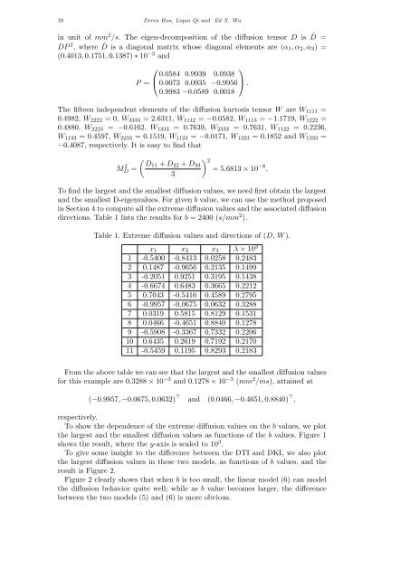
To find the largest and the smallest diffusion values, we need first obtain the largest
and the smallest D-eigenvalues. For given b value, we can use the method proposed
in Section 4 to compute all the extreme diffusion values and the associated diffusion
directions. Table 1 lists the results for b = 2400 (s/mm 2 ).
Table 1. Extreme diffusion values and directions of (D, W ).
x 1 x 2 x 3 λ × 10 3
1 -0.5400 -0.8413 0.0258 0.2483
2 0.1487 -0.9656 0.2135 0.1499
3 -0.2051 0.9251 0.3195 0.1438
4 -0.6674 0.6483 0.3665 0.2212
5 0.7043 -0.5416 0.4589 0.2795
6 -0.9957 -0.0675 0.0632 0.3288
7 0.0319 0.5815 0.8129 0.1531
8 0.0466 -0.4651 0.8840 0.1278
9 -0.5908 -0.3367 0.7332 0.2206
10 0.6435 0.2619 0.7192 0.2170
11 -0.5459 0.1195 0.8293 0.2183
From the above table we can see that the largest and the smallest diffusion values
for this example are 0.3288 × 10 −3 and 0.1278 × 10 −3 (mm 2 /ms), attained at
(−0.9957, −0.0675, 0.0632) ⊤ and (0.0466, −0.4651, 0.8840) ⊤ ,
respectively.
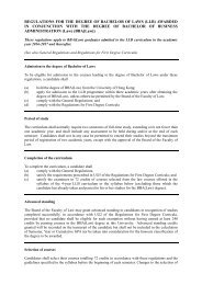
To show the dependence of the extreme diffusion values on the b values, we plot
the largest and the smallest diffusion values as functions of the b values. Figure 1
shows the result, where the y-axis is scaled to 10 3 .
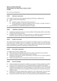
To give some insight to the difference between the DTI and DKI, we also plot
the largest diffusion values in these two models, as functions of b values, and the
result is Figure 2.
Figure 2 clearly shows that when b is too small, the linear model (6) can model
the diffusion behavior quite well; while as b value becomes larger, the difference
between the two models (5) and (6) is more obvious.