RESEARCH ARTICLE Extreme Diffusion Values for non-Gaussian ...

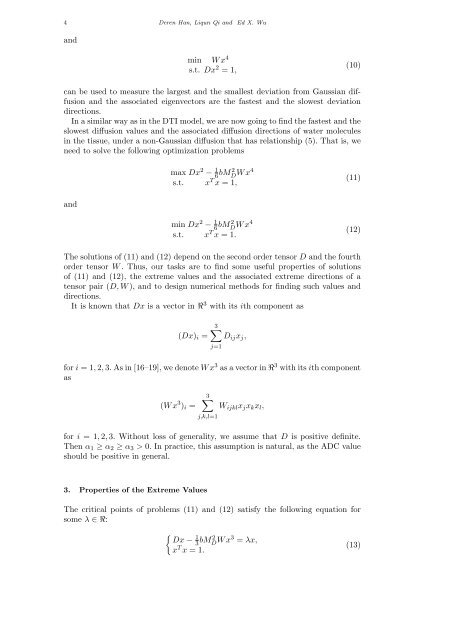
4 Deren Han, Liqun Qi and Ed X. Wu
and
min W x 4
s.t. Dx 2 = 1,
(10)
can be used to measure the largest and the smallest deviation from Gaussian diffusion
and the associated eigenvectors are the fastest and the slowest deviation
directions.
In a similar way as in the DTI model, we are now going to find the fastest and the
slowest diffusion values and the associated diffusion directions of water molecules
in the tissue, under a non-Gaussian diffusion that has relationship (5). That is, we
need to solve the following optimization problems
max Dx 2 − 1 6 bM 2 D W x4
s.t. x T x = 1,
(11)
and
min Dx 2 − 1 6 bM 2 D W x4
s.t. x T x = 1.
(12)
The solutions of (11) and (12) depend on the second order tensor D and the fourth
order tensor W . Thus, our tasks are to find some useful properties of solutions
of (11) and (12), the extreme values and the associated extreme directions of a
tensor pair (D, W ), and to design numerical methods for finding such values and
directions.
It is known that Dx is a vector in R 3 with its ith component as
(Dx) i =
3∑
D ij x j ,
j=1
for i = 1, 2, 3. As in [16–19], we denote W x 3 as a vector in R 3 with its ith component
as
(W x 3 ) i =
3∑
j,k,l=1
W ijkl x j x k x l ,
for i = 1, 2, 3. Without loss of generality, we assume that D is positive definite.
Then α 1 ≥ α 2 ≥ α 3 > 0. In practice, this assumption is natural, as the ADC value
should be positive in general.
3. Properties of the Extreme Values
The critical points of problems (11) and (12) satisfy the following equation for
some λ ∈ R:
{
Dx −
1
3 bM 2 D W x3 = λx,
x T x = 1.
(13)