RESEARCH ARTICLE Extreme Diffusion Values for non-Gaussian ...

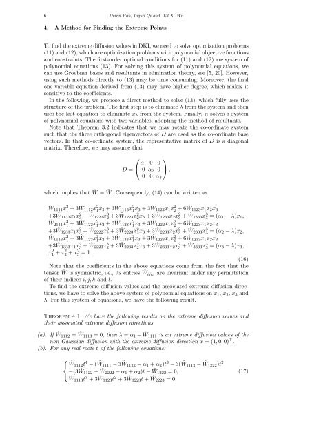
6 Deren Han, Liqun Qi and Ed X. Wu
4. A Method for Finding the Extreme Points
To find the extreme diffusion values in DKI, we need to solve optimization problems
(11) and (12), which are optimization problems with polynomial objective functions
and constraints. The first-order optimal conditions for (11) and (12) are system of
polynomial equations (13). For solving this system of polynomial equations, we
can use Groebner bases and resultants in elimination theory, see [5, 20]. However,
using such methods directly to (13) may be time consuming. Moreover, the final
one variable equation derived from (13) may have higher degree, which makes it
sensitive to the coefficients.
In the following, we propose a direct method to solve (13), which fully uses the
structure of the problem. The first step is to eliminate λ from the system and then
uses the last equation to eliminate x 3 from the system. Finally, it solves a system
of polynomial equations with two variables, adopting the method of resultants.
Note that Theorem 3.2 indicates that we may rotate the co-ordinate system
such that the three orthogonal eigenvectors of D are used as the co-ordinate base
vectors. In that co-ordinate system, the representative matrix of D is a diagonal
matrix. Therefore, we may assume that
D =
⎛
⎝ α ⎞
1 0 0
0 α 2 0 ⎠ ,
0 0 α 3
which implies that Ŵ = ¯W . Consequently, (14) can be written as
Ŵ 1111 x 3 1 + 3Ŵ1112x 2 1 x 2 + 3Ŵ1113x 2 1 x 3 + 3Ŵ1122x 1 x 2 2 + 6Ŵ1123x 1 x 2 x 3
+3Ŵ1133x 1 x 2 3 + Ŵ1222x 3 2 + 3Ŵ1223x 2 2 x 3 + 3Ŵ1233x 2 x 2 3 + Ŵ1333x 3 3 = (α 1 − λ)x 1 ,
Ŵ 2111 x 3 1 + 3Ŵ1122x 2 1 x 2 + 3Ŵ1123x 2 1 x 3 + 3Ŵ1222x 1 x 2 2 + 6Ŵ1223x 1 x 2 x 3
+3Ŵ1233x 1 x 2 3 + Ŵ2222x 3 2 + 3Ŵ2223x 2 2 x 3 + 3Ŵ2233x 2 x 2 3 + Ŵ2333x 3 3 = (α 2 − λ)x 2 ,
Ŵ 1113 x 3 1 + 3Ŵ1123x 2 1 x 2 + 3Ŵ1133x 2 1 x 3 + 3Ŵ1223x 1 x 2 2 + 6Ŵ1233x 1 x 2 x 3
+3Ŵ1333x 1 x 2 3 + Ŵ2223x 3 2 + 3Ŵ2233x 2 2 x 3 + 3Ŵ2333x 2 x 2 3 + Ŵ3333x 3 3 = (α 3 − λ)x 3 ,
x 2 1 + x2 2 + x2 3 = 1. (16)
Note that the coefficients in the above equations come from the fact that the
tensor Ŵ is symmetric, i.e., its entries Ŵijkl are invariant under any permutation
of their indices i, j, k and l.
To find the extreme diffusion values and the associated extreme diffusion directions,
we have to solve the above system of polynomial equations on x 1 , x 2 , x 3 and
λ. For this system of equations, we have the following result.
Theorem 4.1 We have the following results on the extreme diffusion values and
their associated extreme diffusion directions.
(a). If Ŵ 1112 = Ŵ1113 = 0, then λ = α 1 − Ŵ1111 is an extreme diffusion values of the
non-Gaussian diffusion with the extreme diffusion direction x = (1, 0, 0) ⊤ .
(b). For any real roots t of the following equations:
⎧
⎨ Ŵ 1112 t 4 − (Ŵ1111 − 3Ŵ1122 − α 1 + α 2 )t 3 − 3(Ŵ1112 − Ŵ1222)t 2
−(3Ŵ1122 −
⎩
Ŵ2222 − α 1 + α 2 )t − Ŵ1222 = 0,
Ŵ 1113 t 3 + 3Ŵ1123t 2 + 3Ŵ1223t + Ŵ2223 = 0,
(17)