RESEARCH ARTICLE Extreme Diffusion Values for non-Gaussian ...

12 Deren Han, Liqun Qi and Ed X. Wu
in unit of mm 2 /s. The eigen-decomposition of the diffusion tensor D is ˆD =
DP 2 , where ˆD is a diagonal matrix whose diagonal elements are (α 1 , α 2 , α 3 ) =
(1.6928, 1.2448, 1.1936) ∗ 10 −3 and
⎛
⎞
0.0379 −0.9991 0.0174
P = ⎝ −0.9992 −0.0381 −0.0148 ⎠ .
−0.0154 0.0168 0.9997
The fifteen independent elements of the diffusion kurtosis tensor W are W 1111 =
0.1171 × 10 −5 , W 2222 = 0.2665 × 10 −5 , W 3333 = 0.1425 × 10 −5 , W 1112 = −0.0009 ×
10 −5 , W 1113 = 0.0031 × 10 −5 , W 1222 = 0.0026 × 10 −5 , W 2223 = 0.0046 × 10 −5 ,
W 1333 = 0.0044 × 10 −5 , W 2333 = −0.0008 × 10 −5 , W 1122 = 0.0456 × 10 −5 , W 1133 =
0.0348 × 10 −5 , W 2233 = 0.0681 × 10 −5 , W 1123 = 0.0016 × 10 −5 , W 1223 = −0.0015 ×
10 −5 and W 1233 = 0.0013 × 10 −5 , respectively. We can find that
( )
MD 2 D11 + D 22 + D 2
33
=
= 1.8964 × 10 −6 .
3
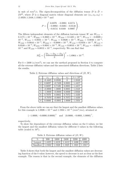
For b = 2400 (s/mm 2 ), we can use the method proposed in Section 4 to compute
all the extreme diffusion values and the associated diffusion directions. Table 2 lists
the results.
Table 2. Extreme diffusion values and directions of (D, W ).
x 1 x 2 x 3 λ × 10 3
1 -0.4485 0.8938 0 1.3349
2 0.6697 -0.7426 0.0001 1.4457
3 0.6697 0.7426 0.0001 1.4457
4 -0.0000 1.0000 0.0001 1.2448
5 -1.0000 -0.0000 0.0000 1.6926
6 0.7070 0.0002 0.7072 1.4430
7 -0.7070 -0.0001 0.7072 1.4430
8 0.0000 -0.0001 1.0000 1.1934
From the above table we can see that the largest and the smallest diffusion values
for this example is 1.6926 × 10 −3 and 1.1934 × 10 −3 (mm 2 /ms), attained at
(−1.0000, −0.0000, 0.0000) ⊤ and (0.0000, −0.0001, 1.0000) ⊤ ,
respectively.
To show the dependence of the extreme diffusion values on the b values, we list
the largest and the smallest diffusion values for different b values in the following
table (scaled to 10 3 ).
Table 3. Extreme diffusion values of (D, W ).
b 800 1600 2400 3200 4000
Largest 1.4425 1.4419 1.4412 1.4406 1.4399
Smallest 1.1932 1.1928 1.1925 1.1921 1.1917
Table 3 shows that both the largest and the smallest diffusion values are decreasing
function of the b value; however, the speed to decrease is not as clear as the first
example. The reason is that in the second example, the elements of the diffusion