Math 312 Lecture Notes Markov Chains - Department of Mathematics

Math 312 Lecture Notes
Markov Chains
Warren Weckesser
Department of Mathematics
Colgate University
Updated, 30 April 2005
Markov Chains
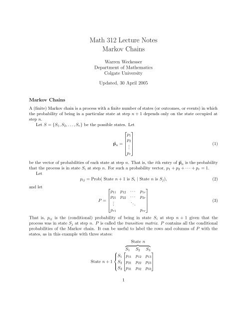
A (finite) Markov chain is a process with a finite number of states (or outcomes, or events) in which
the probability of being in a particular state at step n + 1 depends only on the state occupied at
step n.
Let S = {S 1 , S 2 , . . . , S r } be the possible states. Let
⎡ ⎤
p 1
p 2
⃗p n = ⎢ ⎥
(1)
⎣ . ⎦
p r
be the vector of probabilities of each state at step n. That is, the ith entry of ⃗p n is the probability
that the process is in state S i at step n. For such a probability vector, p 1 + p 2 + · · · + p r = 1.
Let
p ij = Prob( State n + 1 is S i | State n is S j ), (2)
and let
⎡
⎤
p 11 p 12 · · · p 1r
p 21 p 22 · · · p 2r
P = ⎢
⎣
.
. ..
⎥
⎦
p rr
p r1
That is, p ij is the (conditional) probability of being in state S i at step n + 1 given that the
process was in state S j at step n. P is called the transition matrix. P contains all the conditional
probabilities of the Markov chain. It can be useful to label the rows and columns of P with the
states, as in this example with three states:
State n
{ }} {
⎧
S 1 S 2 S
⎡
3
⎤
⎪⎨ S 1 p 11 p 12 p 13
⎢
⎥
State n + 1 S 2 ⎣p 21 p 22 p 23 ⎦
⎪⎩
S 3 p 31 p 32 p 33
1
(3)

The fundamental property of a Markov chain is that
⃗p n+1 = P ⃗p n . (4)
Given an initial probability vector ⃗p 0 , we can determine the probability vector at any step n by
computing the iterates of a linear map.
The information contained in the transition matrix can also be represented in a transition
diagram. In a transition diagram, the states are arranged in a diagram, typically with a “bubble”
around each state. If p ij > 0, then an arrow is drawn from state j to state i, and the arrow is
labeled with p ij . Examples are given in the following discussions.
In these notes, we will consider two special cases of Markov chains: regular Markov chains and
absorbing Markov chains. Generalizations of Markov chains, including continuous time Markov
processes and infinite dimensional Markov processes, are widely studied, but we will not discuss
them in these notes.
Regular Markov Chains
Definition. A Markov chain is a regular Markov chain if some power of the transition matrix has
only positive entries. That is, if we define the (i, j) entry of P n to be p (n)
ij
, then the Markov chain
is regular if there is some n such that p (n)
ij
> 0 for all (i, j).
If a Markov chain is regular, then no matter what the initial state, in n steps there is a positive
probability that the process is in any of the states.
Essential facts about regular Markov chains.
1. P n → W as n → ∞, where W is a constant matrix and all the columns of W are the same.
2. There is a unique probability vector ⃗w such that P ⃗w = ⃗w.
Note:
(a) ⃗w is a fixed point of the linear map ⃗x i+1 = P⃗x i .
(b) ⃗w is an eigenvector associated with the eigenvalue λ = 1. (The claim implies that the
transition matrix P of a regular Markov chain must have the eigenvalue λ = 1. Then ⃗w
is the eigenvector whose entries add up to 1.)
(c) The matrix W is W = [ ⃗w ⃗w · · · ⃗w ] .
3. P n ⃗p 0 → ⃗w as n → ∞ for any initial probability vector ⃗p 0 . Thus ⃗w gives the long-term
probability distribution of the states of the Markov chain.
Example: Sunny or Cloudy. A meteorologist studying the weather in a region decides to
classify each day as simply sunny or cloudy. After analyzing several years of weather records, he
finds:
• the day after a sunny day is sunny 80% of the time, and cloudy 20% of the time; and
• the day after a cloudy day is sunny 60% of the time, and cloudy 40% of the time.
2

We can setup up a Markov chain to model this process. There are just two states: S 1 = sunny,
and S 2 = cloudy. The transition diagram is
and the transition matrix is
0.8 0.2
State 1
Sunny
P =
0.6
State 2
Cloudy
0.4
[ ] 0.8 0.6
. (5)
0.2 0.4
We see that all entries of P are positive, so the Markov chain is regular. (The conditions of the
definition are satisfied when n = 1.)
To find the long-term probabilities of sunny and cloudy days, we must find the eigenvector of
P associated with the eigenvalue λ = 1. We know from Linear Algebra that if ⃗v is an eigenvector,
then so is c⃗v for any constant c ≠ 0. The probability vector ⃗w is the eigenvector that is also a
probability vector. That is, the sum of the entries of the vector ⃗w must be 1.
We solve
P ⃗w = ⃗w
(P − I)⃗w = ⃗0
(6)
Now
P − I =
[ −0.2
] 0.6
0.2 −0.6
If you have recently studied Linear Algebra, you could probably write the answer down with no
further work, but we will show the details here. We form the augmented matrix and use Gaussian
elimination:
⎡
⎤ ⎡
⎤
⎣
−0.2 0.6 . 0
⎦ → ⎣ 1 −3 . 0 ⎦ (8)
0.2 −0.6 . 0 0 0 . 0
which tells us w 1 = 3w 2 , or w 1 = 3s, w 2 = s, where s is arbitrary, or
[ 3
⃗w = s
1]
(7)
(9)
The vector ⃗w must be a probability vector, so w 1 + w 2 = 1. This implies 4s = 1 or s = 1/4. Thus
[ ] 3/4
⃗w = . (10)
1/4
This vector tells us that in the long run, the probability is 3/4 that the process will be in state 1,
and 1/4 that the process will be in state 2. In other words, in the long run 75% of the days are
sunny and 25% of the days are cloudy.
3

Examples: Regular or not
chain is regular.
Here are a few examples of determining whether or not a Markov
1. Suppose the transition matrix is
We find
and, in general,
P =
[ ] 1/3 0
. (11)
2/3 1
[
P 2 (1/3)
=
2 ] [
0
, P 3 (1/3)
=
3 ]
0
(2/3)(1 + 1/3) 1
(2/3)(1 + 1/3 + (1/3) 2 , (12)
) 1
[
P n (1/3)
=
n ]
0
(2/3)(1 + 1/3 + · · · + (1/3) n−1 . (13)
) 1
The upper right entry in P n is 0 for all n, so the Markov chain is not regular.
2. Here’s a simple example that is not regular.
P =
[ ] 0 1
1 0
(14)
Then
P 2 = I, P 3 = P, etc. (15)
Since P n = I if n is even and P n = P if n is odd, P always has two entries that are zero.
Therefore the Markov chain is not regular.
3. Let
⎡
1/5 1/5
⎤
2/5
P = ⎣ 0 2/5 3/5⎦ (16)
4/5 2/5 0
The transition matrix has two entries that are zero, but
⎡
9/25 7/25
⎤
5/25
P 2 = ⎣12/25 10/25 6/25 ⎦ . (17)
4/25 8/25 14/25
Since all the entries of P 2 are positive, the Markov chain is regular.
4

Absorbing Markov Chains
We consider another important class of Markov chains. A state S k of a Markov chain is called
an absorbing state if, once the Markov chains enters the state, it remains there forever. In other
words, the probability of leaving the state is zero. This means p kk = 1, and p jk = 0 for j ≠ k.
A Markov chain is called an absorbing chain if
(i) it has at least one absorbing state; and
(ii) for every state in the chain, the probability of reaching an absorbing state in a finite number
of steps is nonzero.
An essential observation for an absorbing Markov chain is that it will eventually enter an absorbing
state. (This is a consequence of the fact that if a random event has a probability p > 0 of occurring,
then the probability that it does not occur is 1 − p, and the probability that it does not occur in
n trials is (1 − p) n . As n → ∞, the probability that the event does not occur goes to zero.) The
non-absorbing states in an absorbing Markov chain are called transient states.
Suppose an absorbing Markov chain has k absorbing states and l transient states. If, in our set
of states, we list the absorbing states first, we see that the transition matrix has the form
That is, we may partition P as
Absorbing States Transient States
{ }} { { }} {
S 1 S 2 · · · S k S k+1 · · · S
⎡
k+l
⎤
S 1 1 0 · · · 0 p 1,k+1 · · · p 1,k+l
S 2
0 1 . .
.
.
. . .. 0
S k
0 · · · 0 1 p k,k+1 · · · p k,k+l
S k+1
0 · · · · · · 0 p k+1,k+1 · · · p k+1,k+l
⎢
⎥
. ⎣.
. .
. ⎦
S k+l 0 · · · · · · 0 p k+l,k+1 · · · p k+l,k+l
P =
[ ] I R
0 Q
where I is k × k, R is k × l, 0 is l × k and Q is l × l. R gives the probabilities of transitions from
transient states to absorbing states, while Q gives the probabilities of transitions from transient
states to transient states.
Consider the powers of P :
P 2 =
[ ]
I R(I + Q)
0 Q 2 , P 3 =
(18)
[ I R(I + Q + Q 2 ]
)
0 Q 3 , (19)
and, in general,
P n =
[ I R(I + Q + Q 2 + · · · + Q n−1 ] [ ∑
) I R n−1
]
0 Q n =
i=0 Qi
0 Q n , (20)
5

Now I claim that 1
That is, we have
1. Q n → 0 as n → ∞, and
2.
∞∑
Q i = (I − Q) −1 .
i=0
lim P n =
n→∞
[ ]
I R(I − Q)
−1
0 0
The first claim, Q n → 0, means that in the long run, the probability is 0 that the process will be
in a transient state. In other words, the probability is 1 that the process will eventually enter an
absorbing state. We can derive the second claim as follows. Let
Then
QU = Q
U =
(21)
∞∑
Q i = I + Q + Q 2 + · · · (22)
i=0
∞∑
Q i = Q + Q 2 + Q 3 + · · · = (I + Q + Q 2 + Q 3 + · · · ) − I = U − I. (23)
i=0
Then QU = U − I implies
U − UQ = I
U(I − Q) = I
U = (I − Q) −1 ,
(24)
which is the second claim. (The claims can be rigorously justified, but for our purposes, the above
arguments will suffice.)
The matrix R(I − Q) −1 has the following meaning. The column i of R(I − Q) −1 gives the
probabilities of ending up in each of the absorbing states, given that the process started in the i th
transient states.
There is more information that we can glean from (I −Q) −1 . For convenience, call the transient
states T 1 , T 2 , . . . , T l . (So T j = S k+j .) Let V (T i , T j ) be the expected number of times that the
process is in state T i , given that it started in T j . (V stands for the number of “visits”.) Also recall
that Q gives the probabilities of transitions from transient states to transient states, so
I claim that V (T i , T j ) satisfies the following equation:
q ij = Prob( State n + 1 is T i | State n is T j ) (25)
V (T i , T j ) = e ij + q i1 V (T 1 , T j ) + q i2 V (T 2 , T j ) + · · · + q il V (T l , T j ) (26)
where
e ij =
{
1 if i = j
0 otherwise
(27)
1 There is a slight abuse of notation in the formula given. I use the symbol 0 to mean “a matrix of zeros of the
appropriate size”. The two 0’s in the formula are not necessarily the same size. The 0 in the lower left is l × k, while
the 0 in the lower right is l × l.
6

Why Consider just the term q i1 V (T 1 , T j ). Given that the process started in T j , V (T 1 , T j ) gives
the expected number of times that the process will be in T 1 . The number q i1 gives the probability
of making a transition from T 1 to T i . Therefore, the product q i1 V (T 1 , T j ) gives the expected number
of transitions from T 1 to T i , given that the process started in T j . Similarly, q i2 V (T 2 , T j ) gives the
expected number of transitions from T 2 to T i , and so on. Therefore the total number of expected
transition to T i is q i1 V (T 1 , T j ) + q i2 V (T 2 , T j ) + · · · + q il V (T l , T j ).
The expected number of transitions into a state is the same as the expected number of times
that the process is in a state, except in one case. Counting the transitions misses the state in
which the process started, since there is no “transition” into the initial state. This is why the term
e ij is included in (26). When we consider V (T i , T i ), we have to add 1 to the expected number of
transitions into T i to get the correct expected number of times that the process was in T i .
Equation (26) is actually a set of l 2 equations, one for each possible (i, j). In fact, it is just one
component of a matrix equation. Let
⎡
⎤
V (T 1 , T 1 ) V (T 1 , T 2 ) · · · V (T 1 , T l )
V (T 2 , T 1 ) V (T 2 , T 2 )
N = ⎢
⎣
.
.
..
⎥
(28)
⎦
V (T l , T 1 ) V (T l , T l )
Then equation (26) is the (i, j) entry in the matrix equation
(You should check this yourself!) Solving (29) gives
N = I + QN. (29)
N − QN = I
(I − Q)N = I
N = (I − Q) −1 (30)
Thus the (i, j) entry of (I − Q) −1 gives the expected number of times that the process is in the i th
transient state, given that it started in the j th transient state. It follows that the sum of the i th
column of N gives the expected number of times that the process will be in some transient state,
given that the process started in the j th transient state.
Example: The Coin and Die Game. In this game there are two players, Coin and Die. Coin
has a coin, and Die has a single six-sided die. The rules are:
• When it is Coin’s turn, he or she flips the coin. If the coin turns up heads, Coin wins the
game. If the coin turns up tails, it is Die’s turn.
• When it is Die’s turn, he or she rolls the die. If the die turns up 1, Die wins. If the die turns
up 6, it is Coin’s turn. Otherwise, Die rolls again.
When it is Coin’s turn, the probability is 1/2 that Coin will win and 1/2 that it will become Die’s
turn. When it is Die’s turn, the probabilities are
• 1/6 that Die will roll a 1 and win,
7

• 1/6 that Die will roll a 6 and it will become Coin’s turn, and
• 2/3 that Die will roll a 2, 3, 4, or 5 and have another turn.
To describe this process as a Markov chain, we define four states of the process:
• State 1 : Coin has won the game.
• State 2 : Die has won the game.
• State 3 : It is Coin’s turn.
• State 4 : It is Die’s turn.
We represent the possible outcomes in the following transition diagram:
1
State 1
Coin Wins
1/2
State 3
Coin’s Turn
1/2
1/6
1
State 2
Die Wins
1/6
State 4
Die’s Turn
2/3
This is an absorbing Markov chain. The absorbing states are State 1 and State 2, in which one of
the players has won the game, and the transient states are State 3 and State 4.
The transition matrix is
⎡
⎤
⎡
⎤
1 0 . 1/2 0
1 0 1/2 0
P = ⎢0 1 0 1/6
⎥
⎣0 0 0 1/6⎦ = 0 1 . 0 1/6
[ ]
. . . . . . . . . . . . . . . . . .
I R
=
(31)
0 Q
0 0 1/2 2/3 ⎢
⎣
0 0 . 0 1/6⎥
⎦
0 0 . 1/2 2/3
where
We find
R =
[ 1/2 0
]
0 1/6
I − Q =
and Q =
[ ] 0 1/6
. (32)
1/2 2/3
[ ]
1 −1/6
, (33)
−1/2 1/3
8

so
and
N = (I − Q) −1 =
R(I − Q) −1 =
[ ] 4/3 2/3
, (34)
2 4
[ 2/3
] 1/3
1/3 2/3
Recall that the first column of R(I − Q) −1 gives the probabilities of entering State 1 or State 2 if
the process starts in State 3. “Starts in State 3” means Coin goes first, and “State 1” means Coin
wins, so this matrix tells us that if Coin goes first, the probability that Coin will win is 2/3, and
the probability that Die will win is 1/3. Similarly, if Die goes first, the probability that Coin will
win is 1/3, and the probability that Die will win is 2/3.
From (34), we can also conclude the following:
1. If Coin goes first, then the expected number of turns for Coin is 4/3, and the expected
number of turns for Die is 2. Thus the expected total number of turns is 10/3 ≈ 3.33.
2. If Die goes first, then the expected number of turns for Coin is 2/3, and the expected number
of turns for Die is 4. Thus the expected total number of turns is 14/3 ≈ 4.67.
The following table gives the results of our “experiment” with the Coin and Die Game along
with the predictions of the theory. In class, a total of 220 games were played in which Coin went
first. Coin won 138 times, and the total number of turns was 821, for an average of 3.73 turns per
game.
Quantity Predicted Experiment
Percentage Won by Coin 66.7 62.7
Average Number of Turns per Game 3.33 3.73
It appears that in our experiment, Die won more often than predicted by the theory. Presumably
if we played the game a lot more, the experimental results would approach the predicted results.
(35)
9