Nondimensionalize the logistic equation - Department of Mathematics

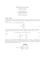
Math 312 Lectures 6 and 7More About NondimensionalizationWarren WeckesserDepartment of MathematicsColgate University31 January 2005In these notes, we first look at an example of nondimensionalizing a differential equation, andthen we look at another application of dimensional analysis.Nondimensionalizing the Logistic EquationRecall the logistic equation:dP(1dt = r − P )P, P (0) = P 0 , (1)Kwhere r > 0 and K > 0 are constants. We’ll follow the steps outlined in the previous lectures tonondimensionalize this differential equation. Table 1 lists the variables and parameters.To create the nondimensional time variable τ, we must divide t by something that has thedimension T . The only choice here is 1/r, so we defineτ =t ( 1r) = rt. (2)To create the nondimensional dependent variable y, we must divide P by something that has thedimension N . We have two choices here, K or P 0 . I’ll use K, and leave the choice of P 0 as anexercise. We havey = P K(3)Variable or Parameter Meaning Dimensiont time TP size of the population Nr per capita growth rate of a small population T −1K carrying capacity NP 0 initial size of the population NTable 1: The list of variables and parameters for the logistic equation, along with their dimensions.T means time and N means an amount or quantity.1

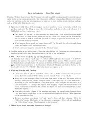
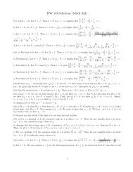
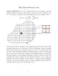
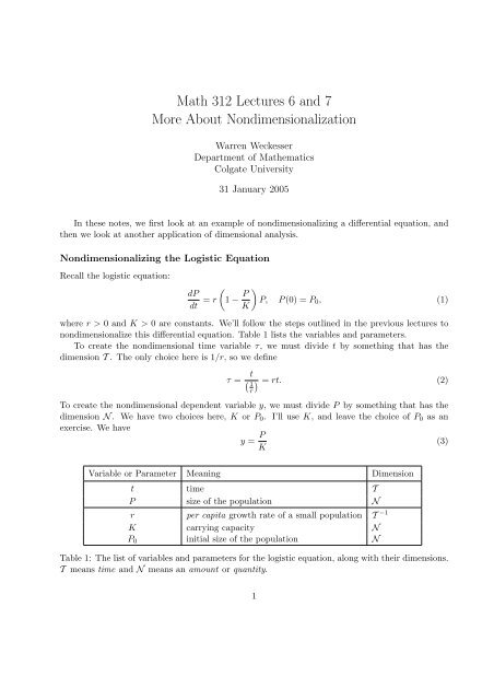
0.3dydt0.20.10-0.2 0 0.2 0.4 0.6 0.8 1 1.2 y-0.1-0.2-0.3Figure 1: The plot of dydtas a function of y for the nondimensional logistic equation (8).For convenience, we also rewrite the definitions of τ and y asBy the chain rule, we haveThen substituting τ and y into (1) givest = τ , P = Ky. (4)rdPdt = d(Ky) dy= rKd(τ/r) dτ . (5)rK dydτ = r(1 − y)Ky, y(0) = P 0K . (6)In the differential equation, the rK factors cancel, so the only parameters left are in the initialcondition. Note that the fraction P 0 /K is nondimensional. We define the new nondimensionalinitial conditiony 0 = P 0(7)Kto arrive at the nondimensional version of the logistic equation:dydτ = (1 − y)y, y(0) = y 0. (8)Now, instead of three dimensional parameters, we have just one nondimensional parameter. Thissimplifies the analysis a bit. At the least, it makes the analysis less cluttered. Figure 1 shows theplot of (1 − y)y, where we can see that there is a stable equilibrium at y = 1. Solutions to thenondimensional equation are shown in Figure 2.2

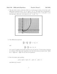
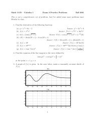
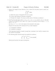
1.5y(t)10.5t0-3 -2 -1 0 1 2 3-0.5Figure 2: The plot of solutions to the nondimensional logistic equation (8) for several differentinitial conditions.How do we interpret the meaning of the nondimensional variables? We defined y = P/K, sothis one is clear. K is a natural unit for the size of the population; y represents the population as afraction of the carrying capacity. The carrying capacity determines an intrinsic unit of measurementfor the population.Can we find a similar interpretation for τ? We formed τ by dividing t by 1/r because thedimension of 1/r is time. Is there some intrinsic “meaning” to 1/r? Consider a small population,where P/K ≪ 1. In this case, the differential equation is approximatelydPdt = rP,and the solution is P (t) = P 0 e rt . Then P (1/r) = P 0 e. Thus we can interpret 1/r as the timerequired for a small population to increase by a factor of e. (This unit of time is similar to the“half-life” of radiactive materials. The half-life is time required for a given sample of the materialto decay to half of the original amount.)3

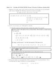
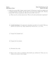
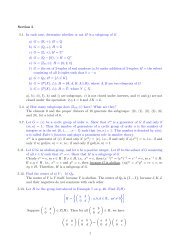
¡¡¡¡¡¡¡¡¡¡¡¡¢¡¢¡¢¡¢¡¢¡¢¡¢¡¢¡¢¡¢¡¢¡¢¡¢¡¢¡¡¡¡¡¡¡¡¡¡¡¡¢¡¢¡¢¡¢¡¢¡¢¡¢¡¢¡¢¡¢¡¢¡¢¡¢¡¢¡¡¡¡¡¡¡¡¡¡¡¡¢¡¢¡¢¡¢¡¢¡¢¡¢¡¢¡¢¡¢¡¢¡¢¡¢¡¢θ 0lmgFigure 3: A pendulum of length l, mass m, acted on by gravity, released from the initial angle θ 0with zero velocity.Parameter Meaning Dimensionl length of the pendulum Lm mass of the pendulum bob Mg gravitational acceleration LT −2θ 0 initial angle 1T period of the oscillation TTable 2: The list of variables and parameters for the logistic equation, along with their dimensions.T means time and N means an amount or quantity.5

We want π to be dimensionless, so we wanta − 2d = 0b + d = 0c = 0(13)This is a linear equation for the unknown a, b, c, and d. Actually, e is also an unknown, but itonly shows up in the exponent of θ 0 , and θ 0 is already dimensionless, so we know e is arbitrary. Itis not difficult to solve the above system of equations, but I will still rewrite in matrix form, andI’ll include e in the system:⎡ ⎤⎡⎤ a ⎡ ⎤1 0 0 −2 0⎢0 1 0 1 0b0⎥⎣0 0 1 0 0⎦⎢c⎥⎣d⎦ = ⎢0⎥⎣0⎦ (14)0 0 0 0 0 0ewhich we can write more concisely asAλ = 0 (15)where A is the dimension matrix and λ is the vector of the powers a, b, c, d, e. Each nontrivialsolution to the linear algebra problem provides a way to combine the dimensional parametersinto a nondimensional product. Note, however, that if λ = [a, b, c, d, e] T is a solution, then so isr [a, b, c, d, e] T = [ra, rb, rc, rd, re] T for any constant r. SinceT ra l rb m rc g rd θ re0 =(T a l b m c g d θ e 0) r, (16)multiples of a solution to (14) do not really identify new combinations of parameters. Thus, all weneed is a set of linearly independent solutions to (14). (To use the lingo from linear algebra, weneed a basis for the null-space of A.) In this case, we see that the system (14) is already in reducedrow echelon form, and the solution can be written⎡ ⎤ ⎡ ⎤2 0−10λ = c 1⎢ ⎥ ⎢0⎥(17)⎢⎣010⎥⎦ + c 2 ⎢ ⎥⎣ ⎦where c 1 and c 2 are arbitrary. Thus a basic for the null-space of A is given by the two vector inthe above solution. So one nondimensional parameter is01and another (which we already knew) isπ 1 = T 2 l −1 m 0 g 1 θ 0 0 = gT 2l(18)π 2 = T 0 l 0 m 0 g 0 θ 1 0 = θ 0 . (19)Presumably there is some relationship among l, m, g, θ 0 , and the period T . We don’t knowwhat it is, so we’ll just assume it can be written in the formf(T, l, m, g, θ 0 ) = 0, (20)6

where f is dimensionally homogeneous. The fundamental result that we will now use is known asthe Buckingham Pi Theorem. It says that a dimensionally homogeneous relation is equivalent toanother relation expressed in terms of only the independent nondimensional parameters π i . Forour example, the Buckingham Pi Theorem implies that there is a function F for whichF (π 1 , π 2 ) = 0. (21)Thus it must be possible to express the relation assumed in (20) in the simpler form( ) gT2F , θ 0 = 0. (22)lEquation (21) is an implicit relation between π 1 and π 2 . We expect that for most values of π 1 andπ 2 , we can solve for π 1 in terms of π 2 . That is, we can write (21) asπ 1 = h(π 2 ) (23)where h is some function. (In principle, the function h exists, but the dimensional analysis performedhere tells us nothing about the nature of h.) Substituting the formulas for π 1 and π 2 into(23) givesgT 2= h(θ 0 ), (24)lorT =√lg h(θ 0) =√lg ĥ(θ 0) (25)where ĥ(θ 0) = √ h(θ 0 ). With this result, we can predict how the period of the oscillation of thependulum depends on the parameters g and l, without actually solving (or even writing down) thedifferential equations that describe the motion.For example, suppose a pendulum of length l 1 has period T 1 when released from angle θ 0 . Ifthe length is doubled and the pendulum is released from the same angle, the new period must beT 2 =√l 2g ĥ(θ 0) =√2l 1g ĥ(θ 0) = √ 2√l 1g ĥ(θ 0) = √ 2 T 1 . (26)Thus, doubling the length should cause the period to increase by a factor of √ 2.We can also compare the behavior of a pendulum on Earth to its behavior on Mars. Thegravitational constant g M on Mars is roughly one-third that of Earth’s gravitational consant g E .If, for a given initial angle θ 0 and length l, the period of the oscillation on Earth is 4 seconds, thenon Mars the period will be√√llT M = ĥ(θ 0 ) =g M g E /3 ĥ(θ 0) = √ √l3 ĥ(θ 0 ) = √ 3 T E = √ 3 4 ≈ 6.93 seconds. (27)g E7