Band Theory, Kittel chapter 7
Band Theory, Kittel chapter 7
Band Theory, Kittel chapter 7

Create successful ePaper yourself
Turn your PDF publications into a flip-book with our unique Google optimized e-Paper software.
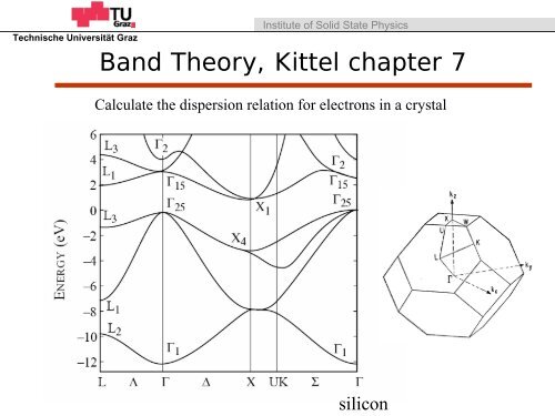
silicon<br />
Institute of Solid State Physics<br />
Technische Universität Graz<br />
<strong>Band</strong> <strong>Theory</strong>, <strong>Kittel</strong> <strong>chapter</strong> 7<br />
Calculate the dispersion relation for electrons in a crystal
Kronig-Penney model<br />
I<br />
II<br />
2 2<br />
d ψ<br />
− + Vx () ψ =<br />
2<br />
2mdx<br />
Eψ<br />
Solutions can be found in region I and region II<br />
Match boundary conditions
Kronig-Penney model<br />
Solutions can be found that are simultaneous eigenfunctions of the<br />
Hamiltonian and the translation operator.<br />
Eigenfunctions of the translation operator can be found in terms of any<br />
two linearly independent solutions. A convenient choice is:<br />
dψ<br />
1<br />
dψ<br />
2<br />
ψ1(0) = 1, (0) = 0, ψ2(0) = 0, (0) = 1.<br />
dx<br />
dx
Kronig-Penney model<br />
for 0 < x < b<br />
ψ ( x) = cos( kx), ψ ( x)<br />
=<br />
1 1 2<br />
for b < x < a<br />
sin( kx<br />
1<br />
)<br />
k<br />
1<br />
k<br />
=<br />
2 mE ( −V1<br />
)<br />
<br />
1 2<br />
ψ<br />
ψ<br />
x k x b kb<br />
k sin( k ( x−b))sin( kb)<br />
1 2 1<br />
1() = cos(<br />
2( − ))cos(<br />
1<br />
) −<br />
,<br />
k2<br />
cos( k ( x−b))sin( kb) sin( k ( x−b))cos( kb)<br />
2 1 2 1<br />
2() x = +<br />
.<br />
k1 k2<br />
k<br />
=<br />
2 mE ( −V2<br />
)<br />
<br />
2 2<br />
Except for the coefficients, these are the same solutions as we found for light<br />
in a layered material.
Kronig-Penney model<br />
at x = a<br />
ψ<br />
ψ<br />
a k a b kb<br />
k sin( k ( a−b))sin( kb)<br />
1 2 1<br />
1() = cos(<br />
2( − ))cos(<br />
1<br />
) −<br />
,<br />
k2<br />
cos( k ( a−b))sin( kb) sin( k ( a−b))cos( kb)<br />
2 1 2 1<br />
2() a = +<br />
.<br />
k1 k2<br />
The translation operator translates the function a distance a.<br />
⎡ψ<br />
( )<br />
( )<br />
1<br />
x + a ⎤ ⎡T11 T12<br />
⎤⎡ψ1<br />
x ⎤<br />
⎢ ⎥=<br />
⎢ ⎥.<br />
ψ ( x + a)<br />
⎢<br />
T T<br />
⎥<br />
⎣ ⎦ ψ ( x)<br />
⎣ 2 ⎦ 21 22 ⎣ 2 ⎦<br />
The elements of the translation operator can be evaluated at x = a.
If |α| > 2, the potential acts like a mirror for electrons<br />
Kronig-Penney model<br />
⎡ dψ<br />
1 ⎤<br />
ψ1<br />
( )<br />
( a) ( a<br />
⎡ψ<br />
)<br />
1<br />
x+<br />
a ⎤ ⎢ dx ⎥⎡ψ1( x)<br />
⎤<br />
⎢ ⎥= ⎢ ⎥⎢ ⎥<br />
⎣ψ2( x+ a)<br />
⎦ ⎢ dψ<br />
2<br />
ψ2<br />
( ) ( )<br />
( x)<br />
ψ2<br />
a a ⎥⎣ ⎦<br />
⎢⎣<br />
dx ⎥⎦<br />
The eigen functions and eigen values are<br />
2 ψ<br />
2( a) 1<br />
ψ<br />
± ( x) = ψ1() x + ψ2(), x λ±= ( α±<br />
δ)<br />
,<br />
dψ<br />
2() a<br />
− ψ<br />
2<br />
1()<br />
a ± δ<br />
dx<br />
δ<br />
2<br />
= α −<br />
dψ<br />
2()<br />
a ⎛k2 k ⎞<br />
1<br />
α = ψ1() a + = 2cos( k2( a−b)<br />
) cos( kb<br />
1 ) − ⎜ + ⎟sin( k2( a−b)<br />
) sin ( kb<br />
1 ).<br />
dx ⎝k1 k2⎠<br />
4
Kronig-Penney model<br />
The eigen values:<br />
1<br />
λ± = ( α±<br />
δ)<br />
2<br />
δ<br />
2<br />
= α −<br />
4<br />
dψ<br />
2()<br />
a ⎛k2 k ⎞<br />
1<br />
α = ψ1() a + = 2cos( k2( a−b)<br />
) cos( kb<br />
1 ) − ⎜ + ⎟sin( k2( a−b)<br />
) sin ( kb<br />
1 ).<br />
dx ⎝k1 k2⎠<br />
If |α| > 2, the eigenvalues are real. The solutions grow or decay exponentially.<br />
If |α| < 2, the eigenvalues are complex and on the unit circle.<br />
ika<br />
λ = e<br />
k<br />
2<br />
1 1 4<br />
tan<br />
⎛ − −α<br />
=± ⎞<br />
a ⎜ α ⎟<br />
⎝ ⎠
Kronig-Penney model<br />
|α| < 2<br />
⎛<br />
tanka =±⎜<br />
⎜<br />
⎝<br />
2<br />
4−α<br />
α<br />
⎞<br />
⎟<br />
⎠
Kronig-Penney model<br />
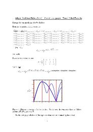
free electrons<br />
(a) The energy-wave number dispersion relation. The dashed line is the Fermi energy. (b) The<br />
density of states. (c) The internal energy density (solid line) and Helmholtz free energy density<br />
(dashed line). (d) The chemical potential (solid line) and the specific heat (dashed line). All of<br />
the plots were drawn for a square wave potential with the parameters: V = 12.5 eV, a =2×10 -<br />
10<br />
m, b =5×10 -11 m, and an electron density of n = 3 electrons/primitive cell.
<strong>Band</strong> structure in 1-D
from Ashcroft and Mermin<br />
Extended, reduced, and<br />
repeated zone schemes<br />
Extended<br />
<br />
k′ = k + k + G<br />
el el photon<br />
Repeated<br />
E ' = E + ω<br />
el el photon<br />
Reduced