Stephens' Kangaroo Rat Survey Report 2007 - Western Riverside ...
Stephens' Kangaroo Rat Survey Report 2007 - Western Riverside ...
Stephens' Kangaroo Rat Survey Report 2007 - Western Riverside ...

Create successful ePaper yourself
Turn your PDF publications into a flip-book with our unique Google optimized e-Paper software.
<strong>Western</strong> <strong>Riverside</strong> County<br />
Multiple Species Habitat Conservation Plan (MSHCP)<br />
Biological Monitoring Program<br />
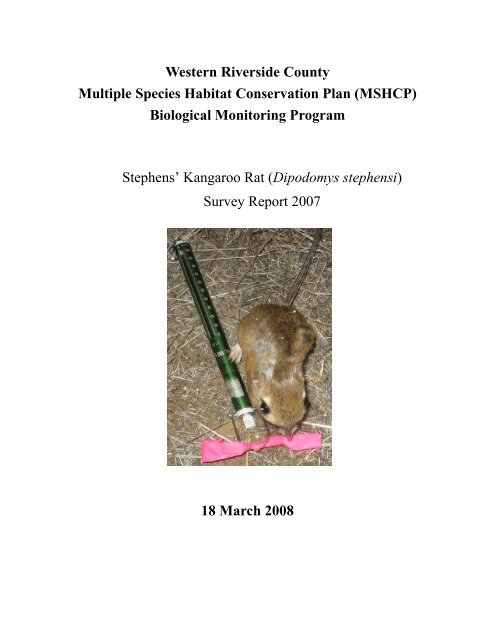
Stephens’ <strong>Kangaroo</strong> <strong>Rat</strong> (Dipodomys stephensi)<br />
<strong>Survey</strong> <strong>Report</strong> <strong>2007</strong><br />
18 March 2008
Stephens’ <strong>Kangaroo</strong> <strong>Rat</strong> <strong>Survey</strong> <strong>Report</strong> <strong>2007</strong><br />
TABLE OF CONTENTS<br />
INTRODUCTION......................................................................................................................... 1<br />
<strong>Survey</strong> Goals....................................................................................................................... 2<br />
METHODS .................................................................................................................................... 2<br />
General Field Protocol ........................................................................................................ 2<br />
5-Night, 7×7 Trapping Efforts ............................................................................................ 3<br />
Full- vs. Partial-Night <strong>Survey</strong>s ........................................................................................... 4<br />
Trap-Initiation..................................................................................................................... 5<br />
Occupancy Estimate............................................................................................................ 5<br />
Incidental Observations – Los Angeles Pocket Mouse <strong>Survey</strong>s......................................... 7<br />
RESULTS ...................................................................................................................................... 7<br />
5-Night, 7×7 Trapping Efforts ............................................................................................ 7<br />
Full- vs. Partial-Night <strong>Survey</strong>s ........................................................................................... 8<br />
Trap-Initiation..................................................................................................................... 9<br />
Occupancy Estimate............................................................................................................ 9<br />
DISCUSSION .............................................................................................................................. 10<br />
Recommendations for Future <strong>Survey</strong>s.............................................................................. 11<br />
REFERENCES............................................................................................................................ 19<br />
LIST OF TABLES AND FIGURES<br />
Table 1. Field staff conducting SKR surveys in <strong>2007</strong>.................................................................... 3<br />
Table 2. Vegetation types used to estimate percent area occupied by SKR at Potrero in October<br />
and November <strong>2007</strong>............................................................................................................ 5<br />
Table 3. Numbers of Stephens’ kangaroo rats captured in Core Areas in <strong>2007</strong>. ........................... 8<br />
Table 4. Numbers of non-target species detected during Stephens’ kangaroo rat surveys in Core<br />
Areas in <strong>2007</strong> ...................................................................................................................... 9<br />
<strong>Western</strong> <strong>Riverside</strong> County MSHCP<br />
Biological Monitoring Program<br />
ii
Stephens’ <strong>Kangaroo</strong> <strong>Rat</strong> <strong>Survey</strong> <strong>Report</strong> <strong>2007</strong><br />
Figure 1. Grid (7x7) locations and Stephens’ kangaroo rat detections at Core Areas, March to<br />
May, <strong>2007</strong>Figure 2. Grid (12x12) locations of Stephens’ kangaroo rat surveys at Potrero<br />
Unit of San Jacinto Wildlife Area, 5 October to 24 November, <strong>2007</strong>............................ 12<br />
Figure 2. Grid (12x12) locations of Stephens’ kangaroo rat surveys at Potrero Unit of San<br />
Jacinto Wildlife Area, 5 October to 24 November, <strong>2007</strong> ............................................... 13<br />
Figure 3. Grid (5x5) locations of Stephens’ kangaroo rat surveys conducted from 15 to 20<br />
October and 6 to 9 November, <strong>2007</strong>Figure 4. 9x9 grids located on Los Angeles pocket<br />
mouse survey sites where Stephens’ kangaroo rat were detected, January to March, <strong>2007</strong>.<br />
........................................................................................................................................... 14<br />
Figure 4. 9x9 grids located on Los Angeles pocket mouse survey sites where Stephens’<br />
kangaroo rat were detected, January to March, <strong>2007</strong>. ...................................................... 15<br />
Figure 5. Capture curves for Stephens’ kangaroo rats trapped on 7x7 grids at 4 Core Areas and<br />
over 5-night efforts when traps were closed at midnight, March - May, <strong>2007</strong>.................16<br />
Figure 6. Capture curves for Stephens’ kangaroo rats surveyed over two 5-night efforts on 7x7<br />
grids checked at Midnight/Dawn vs. Midnight at the Potrero Unit of San Jacinto Wildlife<br />
Area, July & August, <strong>2007</strong> ...............................................................................................16<br />
Figure 7. Capture curves for Stephens’ kangaroo rats surveyed over two 5-night efforts on<br />
12x12 grids at the Potrero Unit of San Jacinto Wildlife Area, September, <strong>2007</strong>.............17<br />
Figure 8. Continuous capture curve combining capture histories of Stephens’ kangaroo rats<br />
trapped over two 5-night efforts on 12x12 grids at the Potrero Unit of San Jacinto<br />
Wildlife Area, September, <strong>2007</strong> .......................................................................................17<br />
Figure 9. Percent slope on 5x5 grids sampled for Stephens’ kangaroo rat at the Potrero Unit of<br />
San Jacinto Wildlife Area, October & November, <strong>2007</strong> ..................................................18<br />
Figure 10. Percent shrub cover on 5x5 grids sampled for Stephens’ kangaroo rat at the Potrero<br />
Unit of San Jacinto Wildlife Area, October & November, <strong>2007</strong>......................................18<br />
LIST OF APPENDICES<br />
Appendix A: Standard Operating Procedure: small mammal trapping ....................................... 21<br />
Appendix B: Habitat Ranking for Selecting <strong>Survey</strong> Sites for Stephens’ <strong>Kangaroo</strong> <strong>Rat</strong> ............. 30<br />
Appendix C: Nightly Unique Captures of Stephens’ <strong>Kangaroo</strong> <strong>Rat</strong> per Grid Using Three<br />
Different <strong>Survey</strong> Designs.................................................................................................. 38<br />
<strong>Western</strong> <strong>Riverside</strong> County MSHCP<br />
Biological Monitoring Program<br />
iii
Stephens’ <strong>Kangaroo</strong> <strong>Rat</strong> <strong>Survey</strong> <strong>Report</strong> <strong>2007</strong><br />
NOTE TO READER:<br />
This report is an account of survey activities undertaken by the Biological Monitoring<br />
Program for the <strong>Western</strong> <strong>Riverside</strong> County Multiple Species Habitat Conservation Plan<br />
(MSHCP). The MSHCP was permitted in June 2004. The Biological Monitoring Program<br />
monitors the distribution and status of the 146 Covered Species within the Conservation Area to<br />
provide information to Permittees, land managers, the public, and the Wildlife Agencies (i.e., the<br />
California Department of Fish and Game and the U.S. Fish and Wildlife Service). Monitoring<br />
Program activities are guided by the MSHCP species objectives for each Covered Species, the<br />
information needs identified in MSHCP Section 5.3 or elsewhere in the document, and the<br />
information needs of the Permittees.<br />
While we have made every effort to accurately represent our data and results, it should be<br />
recognized that our database is still under development. Any reader wishing to make further use<br />
of the information or data provided in this report should contact the Monitoring Program to<br />
ensure that they have access to the best available or most current data.<br />
The primary preparer of this report was the <strong>2007</strong> Mammal Program Lead, Bill Kronland.<br />
If there are any questions about the information provided in this report, please contact the<br />
Monitoring Program Administrator. If you have questions about the MSHCP, please contact the<br />
Executive Director of the <strong>Western</strong> <strong>Riverside</strong> County Regional Conservation Authority (RCA).<br />
For further information on the MSHCP and the RCA, go to www.wrc-rca.org.<br />
Contact Info:<br />
Executive Director<br />
<strong>Western</strong> <strong>Riverside</strong> County<br />
Regional Conservation Authority<br />
4080 Lemon Street, 12th Floor<br />
P.O. Box 1667<br />
<strong>Riverside</strong>, CA 92502-1667<br />
Ph: (951) 955-9700<br />
<strong>Western</strong> <strong>Riverside</strong> County MSHCP<br />
Monitoring Program Administrator<br />
c/o Karin Cleary-Rose<br />
4500 Glenwood Drive, Bldg. C<br />
<strong>Riverside</strong>, CA 92501<br />
Ph: (951) 782-4238<br />
<strong>Western</strong> <strong>Riverside</strong> County MSHCP<br />
Biological Monitoring Program<br />
iv
Stephens’ <strong>Kangaroo</strong> <strong>Rat</strong> <strong>Survey</strong> <strong>Report</strong> <strong>2007</strong><br />
INTRODUCTION<br />
The Stephens’ kangaroo rat (Dipodomys stephensi; “SKR”) is a small fossorial mammal<br />
that is federally endangered and listed by the state of California as threatened. The geographic<br />
range of SKR lies entirely within portions of western <strong>Riverside</strong> and north-central San Diego<br />
Counties, and extends from the Potrero Valley in the north to the Romana Valley in the south,<br />
and from the Anza Valley in the east to the Corona Hills in the west. SKR most often occurs in<br />
open grasslands or sparse shrub-lands with
Stephens’ <strong>Kangaroo</strong> <strong>Rat</strong> <strong>Survey</strong> <strong>Report</strong> <strong>2007</strong><br />
<strong>Survey</strong> strategies of the Biological Monitoring Program in <strong>2007</strong> focused on developing a<br />
sampling protocol that would generate sufficient sample sizes for capture-recapture analyses<br />
(e.g., n ≥ 50) while effectively sampling populations. We also addressed occupancy objectives of<br />
the MSHCP. Specifically, our survey goals and objectives for <strong>2007</strong> were as follows:<br />
<strong>2007</strong> <strong>Survey</strong> Goals and Objectives:<br />
1. Further develop methods suggested by Diffendorfer and Deutschman (2002).<br />
a. Examine utility of data collected from 5-night trapping bouts on 7x7 grids in<br />
cooperation with RCHCA.<br />
b. Compare capture curves and sample sizes from 7x7 grids surveyed during fullnight<br />
vs. partial-night (i.e., closed after midnight check) trapping efforts.<br />
c. Identify whether a trap-initiation period exists (i.e., where SKR capture rates<br />
during the initial nights of a trapping effort are low) at a previously untrapped<br />
site, and how many consecutive trap nights are required before no new SKR<br />
individuals are captured.<br />
d. Assess the use of 12x12 grids to estimate abundance via mark-recapture methods.<br />
2. Incorporate methods suggested by MacKenzie et al. (2002) to estimate SKR occupancy<br />
at the Potrero Unit of the San Jacinto Wildlife Area (Potrero).<br />
a. Test the effectiveness of numerous 5x5 grids to estimate SKR occupancy at<br />
modeled moderate- to high-suitability habitat.<br />
b. Measure vegetation cover at each sample grid to refine the habitat-suitability<br />
model.<br />
METHODS<br />
General Field Protocol<br />
Each <strong>2007</strong> survey effort followed general standard operating procedures developed by<br />
the Biological Monitoring Program for animal handling and data collection (Appendix A). In<br />
general, we used 12″ x 3″ x 3.5″ Sherman live traps modified with paper clips to restrict trap<br />
doors from closing completely and potentially damaging animal tails. We arranged traps in grid<br />
patterns with 15 m spacing, marked each trap station with a labeled pin flag (e.g., “A1”), and<br />
used approximately 1 tbsp of large white Proso millet per trap as bait. We checked traps nightly<br />
between evening and dawn depending on the goals and objectives of individual survey efforts<br />
(see below). We recorded weight (100-g Pesola spring scale), ear length (tip to notch), hind foot<br />
length (Chaetodipus species only), sex, age class (adult, sub adult, juvenile), reproductive<br />
condition (non-reproductive, scrotal, pregnant, lactating, perforate, plugged), capture history<br />
(new, recapture), unique tag ID (when applicable), and trap location of each SKR and non-target<br />
Covered Species (e.g., Dipodomys simulans) upon initial capture in each survey effort. We also<br />
marked the ventral side of all Covered Species with a non-toxic marker and applied either a<br />
uniquely numbered ear tag or injected a Passive Inductive Transmitter (PIT) tag between the<br />
shoulder blades of each SKR (except when estimating occupancy when all SKR were batch<br />
marked only). Animals that were recaptured during a survey effort were released after sex,<br />
reproductive condition, tag ID, and trap location were recorded. We released all non-covered<br />
species (e.g., Peromyscus maniculatus) after recording trap location and species. Processing<br />
times ranged between 30 s and 5 min depending on the presence/absence of tags and the type of<br />
<strong>Western</strong> <strong>Riverside</strong> County MSHCP<br />
Biological Monitoring Program<br />
2
Stephens’ <strong>Kangaroo</strong> <strong>Rat</strong> <strong>Survey</strong> <strong>Report</strong> <strong>2007</strong><br />
mark being applied. Only field personnel with prior animal handling experience and/or<br />
demonstrating proficiency in this area after being trained by experienced Biological Monitoring<br />
Program staff processed animals (Table 1). Program training was conducted in both the field and<br />
office, and focused on proper animal handling, identification, tag application, and standard data<br />
collecting procedures.<br />
Table 1. <strong>Western</strong> <strong>Riverside</strong> County Multiple Species Habitat Conservation Plan Biological Monitoring<br />
Program field staff conducting Stephens’ kangaroo rat surveys in <strong>2007</strong>.<br />
Name Agency Position<br />
Bill Kronland Regional Conservation Authority Mammal Program Lead<br />
Adam Malisch Regional Conservation Authority Lead Biologist<br />
Angie Coates Regional Conservation Authority Field Biologist<br />
Ariana Malone Regional Conservation Authority Field Biologist<br />
Carol Thompson Regional Conservation Authority Field Biologist<br />
Conan Guard Regional Conservation Authority Field Biologist<br />
Debbie De La Torre Regional Conservation Authority Field Biologist<br />
Lynn Miller Regional Conservation Authority Field Biologist<br />
Rosina Gallego Regional Conservation Authority Field Biologist<br />
Ryann Loomis Regional Conservation Authority Field Biologist<br />
Valerie Morgan Regional Conservation Authority Field Biologist<br />
Ricky Escobar Regional Conservation Authority Field Biologist<br />
Espie Sandoval Regional Conservation Authority Field Biologist<br />
Isaac Chellman California Department of Fish and Game Field Biologist<br />
Karin Cleary-Rose U.S. Fish and Wildlife Service Program Coordinator<br />
Amy Rowland 1 Regional Conservation Authority Field Biologist<br />
Andy Boyce 1 Regional Conservation Authority Field Biologist<br />
Christina Greutink 1 Regional Conservation Authority Field Biologist<br />
Lee Ripma 1 Regional Conservation Authority Field Biologist<br />
Theresa Johnson 1 Regional Conservation Authority Field Biologist<br />
Joe Moglia 1 California Department of Fish and Game Field Biologist<br />
1 Data recorder or SKR handling trainee.<br />
5-Night, 7×7 Trapping Efforts<br />
We surveyed for SKR at Silverado Ranch, the Southwestern <strong>Riverside</strong> County Multi-<br />
Species Reserve (MSR), Lake Perris State Park-Davis Unit of the San Jacinto Wildlife Area<br />
(SJWA), and Potrero from 5 March to 16 May <strong>2007</strong> as part of a multi-season effort to examine<br />
sampling methods proposed by Diffendorfer and Deutschman (2002). We surveyed each reserve<br />
non-simultaneously over 5 nights with ten 7x7 grids (90 m x 90 m; 49 traps each) that were<br />
installed and first sampled in summer 2006 (Figure 1). These grids were also sampled in fall and<br />
winter 2006 following the same methods described here, and in coordination with RCHCA<br />
efforts at Estelle Mountain and Steele Peak reserves. Our goal was to examine the utility of data<br />
collected on 7x7 grids to effectively sample populations and generate sufficient sample sizes to<br />
<strong>Western</strong> <strong>Riverside</strong> County MSHCP<br />
Biological Monitoring Program<br />
3
Stephens’ <strong>Kangaroo</strong> <strong>Rat</strong> <strong>Survey</strong> <strong>Report</strong> <strong>2007</strong><br />
model trends across seasons and years with capture-recapture analyses (e.g., closed-capture<br />
models).<br />
Examining seasonal population trends as recommended by Diffendorfer and Deutschman<br />
(2002) required that we survey during winter and spring months when nightly temperatures often<br />
fell below the threshold set by the United States Fish and Wildlife Service (USFWS) 10(a)(1)(A)<br />
permit conditions for SKR. We were also did not use batting (e.g., cotton balls) due to the<br />
tendency of SKR to urinate in traps and render batting material useless. Therefore, we checked<br />
and closed traps at the midpoint of each trap night (e.g., midnight) to avoid nightly temperature<br />
lows and to maintain protocol consistency across seasons.<br />
We marked each SKR ventrally with a non-toxic marker and inserted a sub-cutaneous<br />
PIT tag between the shoulder blades with a 12-gauge hypodermic needle. Batch marking<br />
provided a quick method of determining the proportion of unique individuals captured during a<br />
survey effort, and PIT tags provided a permanent unique mark that can be used to examine longterm<br />
demographic trends (e.g., survivorship, emigration). We batch marked individuals on all but<br />
the final night of an effort, and applied PIT tags to any SKR not already tagged.<br />
We constructed capture curves based on the percent of total unique individuals (M t+1 ;<br />
Cooch and White <strong>2007</strong>) captured per night per site. We considered efforts ineffective at<br />
sampling populations when the percent of total unique individuals captured at a site did not<br />
decrease significantly following the first night of trapping (i.e., low M t+1 to N ratio) and trend<br />
towards 0 by the final night.<br />
Full- vs. Partial-Night <strong>Survey</strong>s<br />
In previous sampling efforts, we sampled SKR during only a portion of the period that<br />
they were trappable, because we closed grids after midnight trap checks. We examined the effect<br />
that attenuating nightly survey efforts had on capture curves and sample size by comparing grids<br />
closed at dawn (full-night) with those closed at midnight (partial-night). We used 7x7 grids that<br />
had been previously sampled in 2006 and <strong>2007</strong> at Potrero (n = 10) and Silverado Ranch (n = 8).<br />
We removed 2 grids from our original sample of 10 at Silverado Ranch because SKR had not<br />
been detected there after 4 survey efforts.<br />
We randomly appointed grids on each reserve to be closed at either dawn or midnight and<br />
began trapping at Silverado Ranch (9 to 14 July) before moving to Potrero (16 to 22 July). We<br />
revisited each grid in identical order after a 1-week rest period and trapped Silverado Ranch from<br />
30 July to 4 August, and Potrero from 7 to 12 August, We accounted for grid bias with a<br />
reciprocal design by keeping grids that had been closed at midnight during the first effort open<br />
until dawn, and closing grids at midnight that had previously been open until dawn. U. S. Fish<br />
and Wildlife Service required that traps be checked twice nightly if they remain open from<br />
sunset to sunrise. We therefore checked all grids at midnight and reset traps on grids that were to<br />
be closed at dawn. We sampled grids over 5 nights during each survey effort, marked SKR<br />
ventrally with a non-toxic marker, and applied a uniquely numbered ear tag (1005-1 Monel,<br />
National Band and Tag Company, Newport, Kentucky) to individuals that did not have a PIT tag.<br />
We pooled data across survey efforts at each site, and compared capture curves of unique SKR<br />
detected (percent of total individuals per night) from grids closed at dawn and midnight.<br />
<strong>Western</strong> <strong>Riverside</strong> County MSHCP<br />
Biological Monitoring Program<br />
4
Stephens’ <strong>Kangaroo</strong> <strong>Rat</strong> <strong>Survey</strong> <strong>Report</strong> <strong>2007</strong><br />
Trap-Initiation<br />
Results from 2006 surveys suggested an initiation period during the early bouts of survey<br />
efforts when SKR were difficult to detect. We examined methods to account for the duration of a<br />
trap initiation period and tested the implementation by sampling a subset of the SKR population<br />
at Potrero that had never been surveyed. This uninitiated population occurred in an area of<br />
Potrero that had previously been closed to surveys due to the potential presence of unexploded<br />
ordnance. We also explored using 12x12 grids to generate larger sample sizes that might be used<br />
to estimate abundance with mark-recapture analyses (i.e., closed-capture models).<br />
We randomly selected 3 survey sites using the Hawth’s Tools extension for ArcMap 9.1<br />
GIS software and a habitat suitability index created by Dudek & Associates (<strong>2007</strong>) based on soil,<br />
vegetation, and slope characteristics known to be favored by SKR (Appendix B). We then<br />
installed a 12x12 grid (165 m x 165 m; 144 traps each) at each selected site with at least 300 m<br />
spacing between grids (Figure 2). Grids were sampled from 5 October to 24 November over two<br />
5-night efforts with a 1-night rest period between surveys. We checked traps at 2300 h and<br />
closed grids after checking traps a second time at dawn. We marked each SKR ventrally with a<br />
non-toxic marker and applied a uniquely numbered ear tag.<br />
We only sampled 2 of 3 grids during the second trapping effort because a gray fox<br />
(Urocyon cinereoargenteus) was observed actively depredating traps during the first midnight<br />
check. The predation resulted in the deaths of 2 SKR and the immediate closure of the grid.<br />
We determined the percent of total unique SKR captured per night by pooling data from<br />
all grids and examined the capture curve of the first 5-night trapping effort for the existence of a<br />
trap-initiation period. An increasing trend in nightly M t+1 would indicate a potential trapinitiation<br />
issue. We then constructed capture curves for each 5-night trapping effort (as well as<br />
the entire 10-night effort, ignoring the 1-night rest period) to determine the number of<br />
consecutive survey nights needed to effectively “trap out” a naïve SKR population. This<br />
threshold would occur when no new SKR were captured for 1 or more nights at a grid where<br />
they had been previously detected in the same trapping effort.<br />
Occupancy Estimate<br />
<strong>Western</strong> <strong>Riverside</strong> County MSHCP species-specific objective 2 for SKR requires the<br />
combined conservation of 3000 ac of occupied habitat in the Potrero Valley and Anza/Cahuilla<br />
Valleys (Dudek & Associates 2003). We addressed this objective using methods suggested by<br />
MacKenzie et al. (2002) to estimate Percent Area Occupied (PAO) of suitable habitat occurring<br />
at Potrero and a contiguous Bureau of Land Management parcel in October and November <strong>2007</strong>.<br />
We identified 2090 ac of moderate- to high-suitability habitat using ArcMap 9.1 GIS software<br />
and the habitat suitability model described above. We modified the habitat index by including<br />
human-disturbed lands (e.g., areas containing woodpiles or old foundations) and coastal sage<br />
scrub/coastal sage scrub-chaparral communities not specifically listed by Dudek & Associates<br />
(<strong>2007</strong>) as moderate- to high-suitability habitat, but with cover density 30%) or low-suitability vegetation<br />
(e.g., shrub density >60%) because Dudek & Associates (<strong>2007</strong>) define these areas as having only<br />
trace densities of SKR (
Stephens’ <strong>Kangaroo</strong> <strong>Rat</strong> <strong>Survey</strong> <strong>Report</strong> <strong>2007</strong><br />
Table 2. Vegetation types not specified by Dudek & Associates (<strong>2007</strong>) as moderate- to high-suitability<br />
habitat, but included within the habitat suitability model used to estimate percent area occupied by Stephens’<br />
kangaroo rat at Potrero in October and November <strong>2007</strong>.<br />
Vegetation Type Cover Density 2 acres<br />
Agriculture 1 - 226.2<br />
California Buckwheat - Brittlebush Moderate 1 11.2<br />
California Annual Grassland Alliance Low to moderate 1 908.8<br />
California Buckwheat - Sugar Bush Association 1 Low 12.7<br />
California Buckwheat - California Sagebrush 1 Low 62.9<br />
California Buckwheat Alliance Moderate 1 21.4<br />
Coast Live Oak / Annual Grass-Herb Association 1 Low to moderate 3.9<br />
Disturbed Shrub and Herb Coastal Sage Scrub 1 Moderate 3.8<br />
Exotic Trees 1 Low to moderate 3.5<br />
Scalebroom - (California Buckwheat - Mexican Elderberry - Mulefat) 1 Low to moderate 51.1<br />
Scalebroom - California Buckwheat Association 1 Low to moderate 26.9<br />
Scalebroom - Mulefat Association 1 Low 0.7<br />
Scalebroom / Menzies' Fiddleneck Association 1 Low to moderate 8.7<br />
Urban Interface 1 - 93.6<br />
Urban or development 1 - 15.4<br />
1 Vegetation types or cover densities not specified as moderate- to high-suitability habitat in Dudek &<br />
Associates (<strong>2007</strong>) model.<br />
2 Moderate cover density = 25% to 60%, low cover density = 30 cm and ≤2 m), and tree<br />
(woody plant >2 m) cover on 0.1-acre circular plots centered on each trapping grid. We further<br />
identified and estimated percent cover of each dominant and co-dominant species occurring<br />
within individual vegetation cover classes. Field personnel initially calibrated their ocular<br />
estimates against point-intercept-derived estimates (two 22 m transects) on each sample plot until<br />
precision and accuracy were each ±5%. We then used point-intercept estimates to recalibrate<br />
ourselves each week on a single plot.<br />
We attempted to estimate PAO and grid-level detection probability based on an<br />
occupancy model in Program MARK (White and Burnham 1999). Occupancy models are similar<br />
to closed-population mark-recapture models, but derive estimates using maximum likelihood<br />
estimation with grid-level presence/absence data rather than individual capture histories<br />
<strong>Western</strong> <strong>Riverside</strong> County MSHCP<br />
Biological Monitoring Program<br />
6
Stephens’ <strong>Kangaroo</strong> <strong>Rat</strong> <strong>Survey</strong> <strong>Report</strong> <strong>2007</strong><br />
(MacKenzie et al. 2002). Furthermore, Program MARK enabled us to include environmental<br />
covariate data (e.g., percent shrub cover) into our estimates, thus providing a more complete<br />
picture of SKR presence/absence. We pooled data from the first 3 nights across efforts and<br />
constructed 9 a priori models that examined the effect of temperature on grid-level detection<br />
probability (p), and shrub cover, ground cover, and percent slope on estimate of occupancy ( Ψˆ ).<br />
Incidental Observations – Los Angeles Pocket Mouse <strong>Survey</strong>s<br />
We detected SKR during monthly surveys for Los Angeles pocket mouse (Perognathus<br />
longimembris brevinasus; “LAPM”) at the Davis Unit of SJWA and Silverado Ranch from<br />
January to March <strong>2007</strong>. We sampled 9x9 grids (80 m x 80 m; 81 traps each) on each reserve for<br />
variable durations depending on immediate survey goals, but never longer than 5 consecutive<br />
nights (Figure 4). We checked traps at the mid-point of each night and marked SKR ventrally<br />
with a non-toxic marker before releasing them. <strong>Survey</strong> methods and results are detailed in the<br />
Los Angeles Pocket Mouse <strong>Survey</strong> <strong>Report</strong> <strong>2007</strong>.<br />
RESULTS<br />
We conducted 18 multiple-night surveys in <strong>2007</strong> and detected 2281 SKR on 87 grids<br />
distributed across 4 Core Areas (Table 3). The Potrero Unit of SJWA (Potrero) was the most<br />
productive area surveyed producing an average 33 (SE = 5) SKR per 7x7 grid per survey.<br />
Silverado Ranch was the least productive site, producing an average 2 (SE = 1) SKR per 7x7 grid<br />
per survey.<br />
We recaptured 187 SKR individuals on our 7x7 grids that were PIT tagged prior to <strong>2007</strong><br />
and applied an additional 420 PIT tags to newly captured animals. We also applied ear tags to<br />
488 newly captured SKR on 7x7 or 12x12 grids, and batch marked 454 unique individuals on<br />
5x5 grids. The number of unique SKR marked during LAPM surveys is unknown because we<br />
surveyed identical grids over multiple efforts and batch marked SKR rather than using unique,<br />
permanent IDs.<br />
We detected 12 non-target species in our traps while surveying for SKR (Table 4). Four<br />
species are Covered under the MSHCP: Dulzura kangaroo rat (Dipodomys simulans), LAPM,<br />
San Diego pocket mouse (Chaetodipus fallax fallax), and San Diego desert wood rat (Neotoma<br />
lepida intermidia). Deer mouse (Peromyscus maniculatus) was the most common non-target<br />
species detected, followed by Dulzura kangaroo rat and San Diego pocket mouse. We also<br />
captured non-mammal species that included western toad (Bufo boreas), California towhee<br />
(Pipilo crissalis), and savannah sparrow (Paaerculus sandwichensis).<br />
5-Night, 7×7 Trapping Efforts<br />
We captured an average 32 (SE = 6) SKR per grid at Potrero, 16 (SE = 5) SKR per grid at<br />
the Southwestern <strong>Riverside</strong> County Multi-Species Reserve (MSR), 9 (SE = 2) SKR per grid at<br />
Lake Perris, and 4 (SE = 2) SKR per grid at Silverado Ranch. We did not detect SKR on 6 grids<br />
at Silverado Ranch and on 1 grid at both Lake Perris and MSR (Appendix C). Our most<br />
productive grid was at Potrero where we detected 68 individual SKR.<br />
Average frequency of initial SKR captures generally fell significantly following the first<br />
survey night and remained comparably low at MSR, Lake Perris, and Silverado Ranch (Figure<br />
5). In contrast, relatively fewer initial captures occurred on the first night at Potrero than at the<br />
<strong>Western</strong> <strong>Riverside</strong> County MSHCP<br />
Biological Monitoring Program<br />
7
Stephens’ <strong>Kangaroo</strong> <strong>Rat</strong> <strong>Survey</strong> <strong>Report</strong> <strong>2007</strong><br />
other 3 sites, and the percent of unique animals detected rose from 26 to 31 between first and<br />
second nights. Furthermore, the trend in initial captures at Potrero was rising by the final night<br />
with 12% of detections on the fourth night and 19% on the fifth.<br />
Table 3. Numbers of Stephens’ kangaroo rats captured in Core Areas in <strong>2007</strong>.<br />
Core Area <strong>Survey</strong> effort Date Grids Sampled SKR Captured 1<br />
5-night, 7x7 effort<br />
5/8 to 5/12, 5/15<br />
to 5/19<br />
10 102<br />
Lake Perris – Davis Unit of<br />
1/22 to 1/26 2 14<br />
San Jacinto Wildlife Area<br />
LAPM<br />
2/20 to 2/22 2 31<br />
3/29 to 3/31 2 21<br />
Southwestern <strong>Riverside</strong><br />
County Multi-Species Reserve<br />
5-night, 7x7 effort 4/24 to 4/28 10 164<br />
5-night, 7x7 effort 4/3 to 4/7 10 42<br />
Silverado Ranch<br />
full- vs. partialsurvey<br />
7/9 to 7/14 8 17<br />
night 7/30 to 8/4 8 11<br />
1/22 to 1/26 2 29<br />
LAPM<br />
2/20 to 2/22 2 24<br />
3/29 to 3/31 2 23<br />
5-night, 7x7 effort 3/20 to 3/24 10 320<br />
Potrero Unit of San Jacinto<br />
Wildlife Area<br />
full- vs. partialsurvey<br />
7/16 to 7/22 10 318<br />
night 8/7 to 8/12 10 363<br />
trap initiation<br />
9/24 to 9/25 3 111<br />
9/30 to 10/5 3 237<br />
occupancy<br />
10/14 to 10/19 20 267<br />
11/6 to 11/9 20 187<br />
1 Number of individual SKR captured per survey. Individuals may have been captured multiple times across efforts.<br />
Full- vs. Partial-Night <strong>Survey</strong>s<br />
We captured 382 SKR at Potrero on grids closed at dawn versus 299 SKR on grids closed<br />
at midnight (Appendix C). At Silverado Ranch we captured 16 SKR on grids closed at dawn<br />
versus 12 SKR on grids closed at midnight. We did not capture SKR on 4 of the 8 grids sampled<br />
at Silverado Ranch and therefore did not construct capture curves for this site because sample<br />
size was too small to provide meaningful insight.<br />
We observed a high capture rate of unique individuals on the first night (59%) with<br />
substantially fewer new animals detected on the final night (10%) during full-night surveys at<br />
Potrero (Figure 6). In contrast, partial-night surveys resulted in relatively fewer captures of<br />
unique individuals on the first night (39%) with only a modest decrease by the final trap night<br />
(10%).<br />
<strong>Western</strong> <strong>Riverside</strong> County MSHCP<br />
Biological Monitoring Program<br />
8
Stephens’ <strong>Kangaroo</strong> <strong>Rat</strong> <strong>Survey</strong> <strong>Report</strong> <strong>2007</strong><br />
Areas in <strong>2007</strong><br />
Table 4. Numbers of non-target species detected during Stephens’ kangaroo rat surveys in Core Areas in <strong>2007</strong>.<br />
Species<br />
Lake<br />
Perris<br />
Southwestern <strong>Riverside</strong><br />
County Multi-Species Reserve<br />
Potrero Unit of San<br />
Jacinto Wildlife Area<br />
Silverado<br />
Ranch<br />
California ground squirrel 1 - 7 -<br />
Dulzura kangaroo rat 1 5 33 68 179<br />
San Diego pocket mouse 1 7 6 25 -<br />
Los Angeles pocket mouse 1 3 - - 18<br />
San Diego wood rat 1 - 1 - -<br />
harvest mouse - 2 3 9<br />
deer mouse 81 36 265 52<br />
cactus mouse - 1 - 1<br />
Audubon’s cottontail - 1 - -<br />
California towhee 1 - - -<br />
savannah sparrow - - 1 -<br />
western toad - 4 1 3<br />
western rattlesnake - 1 - -<br />
1 Covered Species.<br />
Trap-Initiation<br />
The M t+1 capture curve for the initial 5-night trapping effort indicated very low first-night<br />
SKR captures, with slowly increasing captures during nights 2 through 5 (Figure 7), suggesting a<br />
trap-initiation issue. However, full-moon conditions during nights 1 through 3, with cloud cover<br />
during nights 4 and 5, may have affected SKR capture rates.<br />
The most productive night for detecting unique individuals across the entire survey (27%,<br />
n = 69) occurred on the first night of the second 5-night trapping effort (Figure 8) with new SKR<br />
captures declining substantially after this point. We captured 6% and 5% of total unique<br />
individuals across both survey efforts combined on the final 2 nights of the second effort.<br />
Therefore, a single 5-night trapping effort, especially in the presence of a trap-initiation problem,<br />
will likely provide an inadequate index for relative SKR abundance. We were unable to assess<br />
the number of trap nights necessary to “trap out” a local SKR population because of the potential<br />
trap-initiation and moon-phase effects on our capture results.<br />
Occupancy Estimate<br />
We captured SKR on 39 of 40 (97.5%) grids sampled; 27 grids (67.5%) captured ≥ 1<br />
SKR on the first trap night, with the remaining 12 grids capturing SKR on the second night. We<br />
captured no new SKR after the second trap night. We closed 2 grids after the first night; 1<br />
because of gray fox disturbance (but no SKR depredation) and 1 because of compromised crew<br />
safety.<br />
Neither the generalized (i.e., no covariates) nor global (i.e., all covariates) occupancy<br />
models in Program MARK functioned properly because of the very high grid-level capture rates.<br />
Occupancy ( Ψ ˆ = 1.0, SE = 0) and detection probability (p = 1.0, SE = 0.342 E-08) were both<br />
estimated to be 100%, with virtually no variance. Therefore, there was no need to generate an<br />
estimate of occupancy because virtually all of the grids captured SKR within the first 1 or 2 trap<br />
<strong>Western</strong> <strong>Riverside</strong> County MSHCP<br />
Biological Monitoring Program<br />
9
Stephens’ <strong>Kangaroo</strong> <strong>Rat</strong> <strong>Survey</strong> <strong>Report</strong> <strong>2007</strong><br />
nights and the naïve percent of grids occupied (97.5%) provided the best conservative measure<br />
of SKR occupancy.<br />
We were also unable to generate meaningful results from the habitat-covariate models<br />
because all but one of the grids was occupied by SKR. Therefore, we assumed that 97.5% (2038<br />
ac) of the current model’s moderate- to high-suitability SKR habitat at Potrero was occupied as<br />
of October/November <strong>2007</strong>.<br />
Percent shrub ( X = 1.86, 95% CI: 0, 5.88) and ground ( X = 3.03, 95% CI: 0, 11.8) cover<br />
was consistently low and variable across grids with an average percent slope of 2.7 (95% CI: 0,<br />
7.6). Percent ground cover estimates ranged between 0 (n = 2) and 15 (n = 2) with 75% of grids<br />
≤3. Three grids had percent ground cover estimates greater than the upper limit of the 95%<br />
confidence interval and each captured SKR multiple times. The only grid that did not detect SKR<br />
had slope and shrub cover estimates above the upper limit of the 95% confidence intervals<br />
(Figures 9 and 10).<br />
DISCUSSION<br />
We were able to effectively sample SKR populations on 7x7 grids closed at midnight<br />
when animal numbers were moderate to low, but needed the additional effort of both midnight<br />
and dawn checks to effectively sample at Potrero where numbers were high. Midnight and dawn<br />
checks also produced more robust sample sizes, though still too small to estimate population<br />
trends with mark-recapture analyses. Indices may have been appropriate to compare within-year<br />
population trends if midnight/dawn checks were employed across seasons. However, our time<br />
frame for incorporating dawn checks was limited from late spring to early winter because of the<br />
cold-weather risks to SKR. Regardless, abundance indices can not account for animals present<br />
but undetected, and can therefore only provide a relative measure of animals occurring among<br />
sampled sites and can not be used to address site specific density objectives of the MSHCP<br />
(Rosenstock et al. 2002). Furthermore, the effective sampling area was never known during any<br />
of our surveys. Home ranges of sampled SKR occurring near the boundaries of trapping grids<br />
likely included some unknown portion outside of the grid, thus increasing the effective sampling<br />
area by an unknown amount that would result in the overestimation of SKR density (Dice 1938).<br />
Many field and statistical methods have been developed with varying degrees of success<br />
in an attempt to estimate effective sampling area (A). Grid-based estimates of sampling area<br />
often involve the summation of areas covered by trapping grids and a boundary strip whose size<br />
is derived from animal home ranges, distance moved among traps, nested-grid analysis, or trap<br />
data from assessment lines arranged outside of the grid (see Efford 2004 and references therein).<br />
We obtained sample sizes on 12x12 grids sufficient to apply a number of methods to estimate A<br />
and SKR density (e.g., nested grids). However, grid-based estimates often perform poorly<br />
because they tend to rely on separate evaluations of population size and sampling area<br />
(Parmenter et al. 2003). Trapping webs use distance sampling methods to estimate density based<br />
on a distance to detection, and offer promising application to SKR monitoring in that they appear<br />
to perform well when sample size is small (Anderson et al. 1983; Parmenter et al. 2003).<br />
Furthermore, distance sampling incorporates a probability of detection when estimating density,<br />
and can therefore account for individuals present but undetected. One downside to the<br />
<strong>Western</strong> <strong>Riverside</strong> County MSHCP<br />
Biological Monitoring Program<br />
10
Stephens’ <strong>Kangaroo</strong> <strong>Rat</strong> <strong>Survey</strong> <strong>Report</strong> <strong>2007</strong><br />
application of trapping webs is that assumptions of distance sampling must be met, including<br />
100% detection of individuals near the center of the web (Buckland et al. 2001).<br />
Results from our 12x12 grids suggest the existence of an initiation period when SKR<br />
were difficult to detect. Our 7x7 grids also exhibited a similar trend across sites in 2006 and at<br />
Potrero in <strong>2007</strong>. Difficulty in detecting SKR across seasons and sites early in survey efforts<br />
alludes to a behavioral response that may reflect a period when some animals were either<br />
unaware of traps or too wary of them to enter. However, moon visibility may have also affected<br />
detectability as cloud cover increased and the moon began to wane considerably between efforts.<br />
We were able to account for the period of low detectability by sampling 12x12 grids over 2<br />
consecutive 5-night efforts, but believe that additional surveys were needed to definitively define<br />
a period of trap initiation.<br />
Our occupancy estimate relied on grid-level detections and was less affected by<br />
individual SKR trap behavior. Occupancy of SKR on moderate- and high-suitability habitat<br />
occurring at Potrero was high and this location alone accounted for 68% of the conservation goal<br />
stated in Species Objective 2 (i.e., 2038 ac were documented as occupied, out of a minimum goal<br />
of 3000 ac). However, our habitat-suitability model did not accurately account for habitat created<br />
by the 2006 Esperanza Fire, and we suspect that SKR occupy a greater proportion of Potrero<br />
than our estimate suggests.<br />
Habitat suitability appears to be ideal for SKR at Potrero given the high trap success of<br />
each of our surveys there in <strong>2007</strong>. The Esperanza Fire of 2006 greatly reduced shrub and ground<br />
cover densities, and created a landscape with a relatively homogenous vegetation structure.<br />
Indeed, the burn had reduced cover on our grid with the greatest shrub density from 25-40%<br />
(based on pre-fire GIS imagery) to 10% and we never observed total vegetation cover >17%. We<br />
expect that SKR habitat quality at Potrero will begin to diminish as pre-fire vegetation structures<br />
return. Until Potrero enters into more mature post-fire seral stages, occupancy studies based on<br />
habitat-suitability models that incorporate pre-fire vegetation attributes will likely underestimate<br />
SKR distribution.<br />
Recommendations for Future <strong>Survey</strong>s<br />
We will continue to address SKR occupancy objectives in 2008 by sampling 5x5 grids at<br />
Potrero using a habitat suitability model that accounts for habitat created by the 2006 Esperanza<br />
Fire. We will base our model on Dudek & Associates (<strong>2007</strong>) definitions of moderate- to highsuitability<br />
soil and slope but ignore vegetation attributes, thus accounting for potentially<br />
occupied habitat that was previously thought to contain vegetation cover too dense for SKR. We<br />
will also sample 5x5 grids in the Anza/Cahuilla Valleys according to the above habitat-suitability<br />
model, but incorporate moderate- to high- suitability vegetation cover since there will not be a<br />
need to account for habitat created by recent fire. Finally, we will test our habitat models by<br />
estimating vegetation cover on 5x5 grids and including estimates as covariates in closed-capture<br />
occupancy models.<br />
We will also further examine methods of deriving point estimates of abundance to<br />
address density objectives at Potrero and Anza/Cahuilla Valleys. We will examine the use of<br />
trapping webs as a means of estimating density and compare results with estimates derived from<br />
our 12x12 grids in <strong>2007</strong>.<br />
<strong>Western</strong> <strong>Riverside</strong> County MSHCP<br />
Biological Monitoring Program<br />
11
Figure 1. Grid (7x7) locations and <strong>Stephens'</strong> kangaroo rat detections at Core Areas, March to May, <strong>2007</strong>.<br />
Lake Perris/<br />
Davis Unit<br />
San Jacinto Wildlife Area<br />
Potrero Unit<br />
San Jacinto Wildlife Area<br />
Southwest <strong>Riverside</strong> County<br />
Multispecies Reserve<br />
Silverado Ranch<br />
Legend<br />
SKR Not Detected<br />
µ<br />
SKR Detected<br />
Highways<br />
Lakes<br />
Conservation Area<br />
5<br />
Planning Area Boundary<br />
0 10 20 30 40<br />
Km<br />
Date: 08 January 2008<br />
Created By: Bill Kronland<br />
UTM Nad 83 Zone 11<br />
MSHCP Biological Monitoring Program
Figure 2. Grid (12x12) locations of <strong>Stephens'</strong> kangaroo rat surveys at Potrero Unit of San Jacinto Wildlife Area, 5 October<br />
to 24 November <strong>2007</strong>.<br />
µ<br />
Date: 17 January 2008<br />
Created By: Bill Kronland<br />
UTM Nad 83 Zone 11<br />
MSHCP Biological Monitoring Program
Figure 3. Grid (5x5) locations of <strong>Stephens'</strong> kangaroo rat surveys conducted from 15 to 20 October and 6 to 9 November <strong>2007</strong>.<br />
")<br />
")<br />
")<br />
")<br />
")<br />
")<br />
")<br />
")<br />
")<br />
")<br />
")<br />
")<br />
")<br />
")<br />
")<br />
")<br />
")<br />
")<br />
")<br />
")<br />
")<br />
")<br />
")<br />
")<br />
")<br />
")<br />
")<br />
")<br />
")<br />
")<br />
")<br />
")<br />
")<br />
")<br />
") ")<br />
") ")<br />
")<br />
")<br />
Legend<br />
") 15 to 20 of October<br />
") 6 to 9 of November<br />
Suitable Habitat<br />
Conservation Area Boundary<br />
µ<br />
0 0.5 1 2<br />
Km<br />
Date: 17 January 2008<br />
Created By: Bill Kronland<br />
UTM Nad 83 Zone 11<br />
MSHCP Biological Monitoring Program
Figure 4. 9x9 grids located on Los Angeles pocket mouse survey sites where<br />
<strong>Stephens'</strong> kangaroo rat were detected, January to March, <strong>2007</strong><br />
Davis Unit of San Jacinto Wildlife Area<br />
0 0.5 1 2 3<br />
Km<br />
Silverado Ranch<br />
0 0.5<br />
1 2<br />
Km<br />
Legend<br />
9x9 LAPM Grids<br />
Highways<br />
Lakes<br />
Conservation Area<br />
Planning Area Boundary<br />
µ<br />
Date: 17 January 2008<br />
Created By: Bill Kronland<br />
UTM Nad 83 Zone 11<br />
MSHCP Biological Monitoring Program
Stephens’ <strong>Kangaroo</strong> <strong>Rat</strong> <strong>Survey</strong> <strong>Report</strong> <strong>2007</strong><br />
Percent of total unique <strong>Stephens'</strong> kangaroo rat captures<br />
0.7<br />
0.6<br />
0.5<br />
0.4<br />
0.3<br />
0.2<br />
0.1<br />
0.0<br />
Multi Species Reserve<br />
Potrero<br />
Silverado Ranch<br />
Lake Perris<br />
1 2 3 4 5<br />
<strong>Survey</strong> Night<br />
Figure 5. Capture curves for <strong>Stephens'</strong> kangaroo rat trapped on 7x7 grids at 4<br />
Core Areas over 5 nights when traps were closed at midnight, March - May, <strong>2007</strong>.<br />
Percent of total unique <strong>Stephens'</strong> kangaroo rat captures<br />
0.7<br />
0.6<br />
0.5<br />
0.4<br />
0.3<br />
0.2<br />
0.1<br />
0.0<br />
1 2 3 4 5<br />
<strong>Survey</strong> Night<br />
Midnight/Dawn Check<br />
Midnight Check<br />
Figure 6. Capture curves for <strong>Stephens'</strong> kangaroo rats surveyed over two 5-night<br />
efforts on 7x7 grids checked at Midnight/Dawn vs. Midnight at the Potrero Unit<br />
of San Jacinto Wildlife Area, July & August, <strong>2007</strong>.<br />
<strong>Western</strong> <strong>Riverside</strong> County MSHCP<br />
Biological Monitoring Program<br />
16
Stephens’ <strong>Kangaroo</strong> <strong>Rat</strong> <strong>Survey</strong> <strong>Report</strong> <strong>2007</strong><br />
Percent of total unique <strong>Stephens'</strong> kangaroo rat captures<br />
0.7<br />
0.6<br />
0.5<br />
0.4<br />
0.3<br />
0.2<br />
0.1<br />
0.0<br />
1st effort<br />
2nd effort<br />
1 2 3 4 5<br />
<strong>Survey</strong> Night<br />
Figure 7. Capture curves for <strong>Stephens'</strong> kangaroo rats surveyed over two 5-night<br />
efforts on 12x12 grids at the PotreroUnit of San Jacinto Wildlife Area, September,<br />
<strong>2007</strong>.<br />
Percent of total unique Stephen's kangaroo rat captures<br />
0.30<br />
0.25<br />
0.20<br />
0.15<br />
0.10<br />
0.05<br />
0.00<br />
Traps closed<br />
for 1 night<br />
1 2 3 4 5 6 7 8 9 10 11<br />
<strong>Survey</strong> Night<br />
Figure 8. Continuous capture curve combining capture histories of <strong>Stephens'</strong><br />
kangaroo rat trapped over two 5-night efforts on 12x12 grids at the Potrero Unit<br />
of San Jacinto Wildlife Area, September, <strong>2007</strong>.<br />
<strong>Western</strong> <strong>Riverside</strong> County MSHCP<br />
Biological Monitoring Program<br />
17
Stephens’ <strong>Kangaroo</strong> <strong>Rat</strong> <strong>Survey</strong> <strong>Report</strong> <strong>2007</strong><br />
10 No SKR<br />
Detected<br />
8<br />
Percent Slope<br />
6<br />
4<br />
2<br />
0<br />
5 10 15 20 25 30 35 40<br />
Grid<br />
Figure 9. Percent slope on 5x5 grids sampled for <strong>Stephens'</strong> kangaroo rat<br />
at the Potrero Unit of San Jacinto Wildlife Area, October & Novermber, <strong>2007</strong><br />
10<br />
No SKR<br />
Detected<br />
8<br />
Percent shrub cover<br />
6<br />
4<br />
2<br />
0<br />
5 10 15 20 25 30 35 40<br />
Grid<br />
Figure 10. Percent shrub cover on 5x5 grids sampled for <strong>Stephens'</strong> kangaroo rat<br />
<strong>Western</strong> <strong>Riverside</strong> County MSHCP<br />
Biological Monitoring Program<br />
18
Stephens’ <strong>Kangaroo</strong> <strong>Rat</strong> <strong>Survey</strong> <strong>Report</strong> <strong>2007</strong><br />
REFERENCES<br />
Anderson, D.R, K.P. Burnham, G.C. White, and D.L. Otis. 1983. Density estimation of smallmammal<br />
populations using a trapping web and distance sampling methods. Ecology<br />
64:674-680.<br />
Buckland, S.T., D.R. Anderson, K.P. Burnham, J.L. Laake, D.L. Borchers, and L. Thomas. 2001.<br />
Introduction to Distance Sampling: estimating abundance of biological populations (2 nd<br />
edition). Oxford University Pres, Inc, New York, New York, USA.<br />
Burnham, K.P., and D.R. Anderson. 2002. Model selection and multimodel inference: a practical<br />
information-theoretic approach. 2 nd Edition. Springer-Verlag, New York, New York,<br />
USA.<br />
Cooch, E.G., and G.C. White. <strong>2007</strong>. Program MARK: a gentle introduction (6 th edition).<br />
Dice, L.R. 1938. Some census methods for mammals. Journal of Wildlife management 2:119-<br />
130.<br />
Diffendorfer, J.E., and D.H. Deutschman. 2002. Monitoring the Stephens’ kangaroo rat: An<br />
analysis of Monitoring Methods And Recommendations For Future Monitoring.<br />
Department of Biology San Diego State University.<br />
Dudek & Associates. 2003. <strong>Western</strong> <strong>Riverside</strong> County Multiple Species Habitat Conservation<br />
Plan (MSHCP). Final MSCHSP, volumes I and II. Prepared for County of <strong>Riverside</strong><br />
Transportation and lands Management Agency by Dudek & Associates, Inc. Approved<br />
June 17, 2003.<br />
Dudek & Associates. <strong>2007</strong>. Stephens’ kangaroo rat habitat management and monitoring plan &<br />
fire management plan for RCHCA lands in the Lake Mathews and Steele Peak Reserves<br />
by Dudek & Associates, Inc. June 21, <strong>2007</strong>.<br />
Efford, M.G. 2004. Density estimation in live-trapping studies. Oikos 106:598-610.<br />
Hallet, J.G., M.A. O’Connell, G.O. Sanders, and J. Seidensticker. 1991 Comparison of<br />
population estimators for medium-sized mammals. Jounal of Wildlife Management<br />
55:81-93.<br />
MacKenzie, D.I., J.D. Nichols, G.B Lachman, S. Droege, J.A. Royle, and C. A. Langtimm. 2002.<br />
Estimating site occupancy rates when detection probabilities are less than one. Ecology<br />
83:2248-2255.<br />
MacKenzie, D.I., and J.A. Royle. 2005. Designing occupancy studies: general advice and<br />
allocating survey effort. Journal of Applied Ecology 42:1105-1.<br />
McKelvey, K.S., and D.E. Pearson. 2001. Population estimation with sparse data: the role of<br />
estimators versus indices revisited. Canadian Journal of Zoology 79:1754-1765.<br />
O’Farrell, M.J. 1990. Stephens kangaroo rat: natural history, distribution, and current status. In<br />
P.J. Bryant and J. Remington (eds.) Memoirs of the Natural History Foundation of<br />
Orange County 3:77-84.<br />
<strong>Western</strong> <strong>Riverside</strong> County MSHCP<br />
Biological Monitoring Program<br />
19
Stephens’ <strong>Kangaroo</strong> <strong>Rat</strong> <strong>Survey</strong> <strong>Report</strong> <strong>2007</strong><br />
Parmenter, R.R., T.L. Yates, D.R. Anderson, K.P. Burnham, J.L. Dunnum, A.B. Franklin, M.T.<br />
Friggnes, B.C. Lubow, M. Miller, G.S. Olson, C. A. Parmenter, J. Pollard, E. Rexstad,<br />
T.M. Shenk, T.R. Stanley, and G.C. White. 2003. Small-mammal density estimation: a<br />
field comparison of grid-based vs. web-based density estimators. Ecological Monographs<br />
73:1-26.<br />
<strong>Riverside</strong> County Habitat Conservation Agency. 1996. Habitat Conservation Plan for the<br />
Stephens kangaroo rat in <strong>Western</strong> <strong>Riverside</strong> County, California.<br />
Rosenstock, S.S., D.R. Anderson, K.M. Giesen, T. Leukering, and M.F. Carter. 2002. Landbird<br />
counting techniques: current practices and an alternative. The Auk 119:46-53.<br />
White, G.C., and K.P. Burnham. 1999. Program MARK: survival estimation from populations of<br />
marked animals. Bid Study 46 Supplement: 120-138. Downloaded June, <strong>2007</strong>.<br />
<strong>Western</strong> <strong>Riverside</strong> County MSHCP<br />
Biological Monitoring Program<br />
20
Appendix A:<br />
<strong>Western</strong> <strong>Riverside</strong> County MSHCP Monitoring Program<br />
Standard Operating Procedures: Small Mammal Trapping<br />
These are the standard procedures developed by the <strong>Western</strong> <strong>Riverside</strong> County<br />
MSHCP Biological Monitoring Program for trapping small mammals covered by the<br />
Conservation Plan. Individual projects may have specific procedures and requirements that<br />
vary from those described here. Variations from these standard procedures will be described<br />
in the Methods section of individual project protocols.<br />
I. Site Selection<br />
Site selection criteria will be project specific, but generally involve the use of<br />
Geographic Information Systems (GIS) software (e.g. ArcGIS) to generate random points<br />
based on the current available knowledge of target species occurrence. Universal Transverse<br />
Mercator (UTM) coordinates will be assigned to each random point and field crews will use<br />
a Global Positioning System (GPS) unit to navigate to each site and verify that they conform<br />
to individual project selection criteria (e.g. species specific suitable habitat). Grids will be<br />
placed at each random point and consist of only one vegetation community (e.g. grassland)<br />
and soil type (e.g. sandy loam) specific to the target species to be surveyed. Grids will also be<br />
placed at least 100 m from each other and at least 70 m from vegetation communities that<br />
differ from those found on the grid site to avoid edge effects.<br />
II. Setting out Trap Lines<br />
Equipment:<br />
Modified Sherman traps<br />
Millet<br />
List of random UTM points<br />
Ant powder<br />
Transect tape 100m<br />
Flagging/Pin flags<br />
Sharpie pens<br />
Trap carrying bags<br />
Handheld GPS unit/ Compass<br />
Trash bags<br />
Trap Grid Layout: Grids will vary in size according to project specific goals, but will be<br />
installed following identical procedures regardless of design. Grids will be placed so that the<br />
area sampled comprises a homogenous vegetation community with random points<br />
representing southwest corners. We will adjust grid corners and record the new UTM<br />
coordinates in the event that the random point would result in a grid footprint covering<br />
multiple vegetation types. Diagonal distance between corners will be measured to ensure the<br />
gird is square (a 2 + b 2 = c 2 ), and the north-south and east-west lines will be marked with 100-<br />
m tapes. Pin-flags will be labeled and placed according to location within the grid and project<br />
specific intervals (e.g. SKR = 15 m). Trap lines will be labeled alphabetically and increasing<br />
eastward, with trap stations within a line labeled numerically (e.g. A1, A2…A7) and<br />
increasing northward (Figure 1). Note: the number of trap lines within a grid and the number<br />
of stations on a line will differ according to project specific goals.<br />
<strong>Western</strong> <strong>Riverside</strong> County MSHCP<br />
Biological Monitoring Program<br />
21
Trap Placement and Setting: Unfold the trap and push the front door until it engages with<br />
the treadle tab. The front door can easily be found by noticing that there is a crease on the left<br />
side of the trap when the door is facing you. There is also a “lip” at the top of the same side.<br />
Lightly tap on the side or bottom of trap. A light tap will be about as hard as if you<br />
were trying to make a spider fall off the side of the trap. If the trap is set properly the door<br />
should snap shut, if it does not, adjust the sensitivity of the trap by pulling the tab forward or<br />
pushing it backward. Pushing back will make the door more sensitive, a forward pull will<br />
make it less sensitive. Please ask if you cannot find the tab.<br />
Place the trap on the ground at the station with the opening facing northward once<br />
you are sure the sensitivity is correct (placing all the traps facing the same direction reduces<br />
the number of variables). Traps should be placed on a level surface so that the trap does not<br />
teeter and the trap entrance is flush with the ground. Use your boot to scrape out an even<br />
space if necessary. Traps should be placed parallel to the trap line as indicated in the trap<br />
placement diagram (Figure 1). Take about 1 tablespoon of millet and toss most of it into the<br />
trap. Make sure that the millet is in the back of the trap, behind the treadle; otherwise an<br />
animal is likely to be too close to the door when it shuts and damage its tail<br />
A7<br />
C7<br />
D7<br />
G7<br />
North<br />
A1<br />
C1<br />
D1<br />
G1<br />
East<br />
Figure 1.Grid design (7x7) for trapping small mammals. Boxes represent<br />
individual traps and arrows indicate direction that open doors face. Traps are<br />
labeled alphabetically and increasing to the east, numerically and increasing to the<br />
north.<br />
<strong>Western</strong> <strong>Riverside</strong> County MSHCP<br />
Biological Monitoring Program<br />
22
Ant Caution: Ants can kill animals in a trap. Sprinkle provided ant powder liberally under<br />
and in front of traps ff ants are present. Make sure that there are no ants inside the trap before<br />
you rebait it. If you are doing the last trap check of the day/night and there are ants, apply ant<br />
powder unless the grid is being closed. Do not set a trap if the ants are particularly thick and<br />
you feel they are too numerous for the powder to be effective. Be sure to record that the trap<br />
was not set.<br />
III. Checking Traps<br />
Note: All of the procedures described below require training and experience. If you<br />
are not comfortable with the training you have received, or you are fearful that the<br />
methodologies used at your last job are not the ones used here, it is your responsibility to<br />
alert the Mammal Program Lead (Bill) or the Monitoring Program Coordinator (Karin). If<br />
you are scheduled for an activity you do not feel qualified to conduct, alert Karin or Bill as<br />
soon as possible. Do not ever conduct a procedure you are not comfortable with.<br />
Equipment per handler:<br />
1 Headlamp per person<br />
3 Pesola® Scales: 20g, 100g and 300g<br />
2 Rulers (1 short 1 long, 0 at edge)<br />
1 Kestrel per handler<br />
1 Manicure scissors for hair clipping<br />
4 Animal handling bags (Ziplock®)<br />
Datasheets (>2 per grid, extras better)<br />
Grid quality control sheets (>1 per grid)<br />
Animal Mortality Record<br />
Mag light flash light<br />
Clipboard 1 per recorder<br />
Several pens<br />
Species field guide/key<br />
Digital camera<br />
Waste bags for used millet<br />
Ant powder (pre approved only)<br />
Backpack<br />
Extra batteries<br />
Traps will be checked either once or twice per night. The first check (i.e. midnight<br />
check) will be approximately 5 hours after sunset, the second check will be just before dawn.<br />
Traps may be closed after the midnight check, but the midnight check can not be skipped in<br />
favor of a morning only check.<br />
While checking trap lines, note pin-flag number and whether each trap was open,<br />
closed and empty, or closed with a capture. Make note of the status of each trap in the<br />
appropriate box on your trap-check quality control sheet to ensure that no traps are missed.<br />
Mark “O” for open traps, “C” for closed with no capture, “R” for robbed traps, (traps that are<br />
open with no bait inside), and use the four-letter species alpha code for traps closed with an<br />
animal inside. Be sure to physically pick-up each trap to check for bait and ensure that<br />
treadles are set properly. Only record the status of the traps you or your handling/recording<br />
partner checked. Adjust the treadle on robbed traps.<br />
When there is no animal in the trap: If the trap is open, visually check to see there is not a<br />
pocket mouse in the trap. We have captured several pocket mice in open traps when a<br />
surveyor picked up the trap. Additionally, place your hand inside the trap and push the<br />
treadle to the bottom of the trap to ensure that no mice are hiding under the treadle. Never<br />
close a trap without looking inside and checking the treadle first.<br />
<strong>Western</strong> <strong>Riverside</strong> County MSHCP<br />
Biological Monitoring Program<br />
23
Pick up all open traps and dispose of the bait in your waste bag if the grid is being<br />
closed, otherwise reset and bait traps if another check is to occur later that night. Dispose of<br />
excess bait and place closed, empty traps perpendicular to the trap line if it is the final gird<br />
check of the night and grids will be opened the next day.<br />
Pick-up closed traps and gently shake with the door facing upwards so that the<br />
contents move to the back of the trap. This will ensure that very small animals (e.g. pocket<br />
mouse) will not be crushed when you open the trap door. Slowly open traps that seem too<br />
light to contain an animal to ensure that a pocket mouse or small Peromyscus is not inside.<br />
Gently depress the treadle to check for animals underneath. Harvest mice, pocket mice and<br />
determined Peromyscus fit easily under the treadle. Fold traps and put them into a trap bag,<br />
or return it to the trap station as appropriate if you are absolutely certain that they contain no<br />
animals.<br />
When there is an animal in the trap: If the door is closed pick up the trap and take notice of<br />
the weight. If it feels like an animal is inside follow the directions below. Use caution as<br />
occasionally non-mammal species may be captured. See rattlesnakes below.<br />
To remove the mammal from the trap, hold the trap parallel to your body, door facing<br />
upward and the side of the trap with the split panel facing you. One hand should be on each<br />
side of the trap. Your right hand will be holding the bottom of the trap. Place a Ziplock® bag<br />
over the top of the trap. Pull the crease of the bag against the inside right corner of the trap.<br />
Wrap the excess portion of the bag around the trap away from you and hold it securely<br />
against the trap with your right hand. Open and extend the bag so that the animal will easily<br />
fall into it. Gently shake the trap so that animal moves to the back of the trap and will not be<br />
crushed by the door as you open it inwards. With your right hand through the plastic bag,<br />
open and hold the trap door. Invert the trap quickly and firmly with a downward shake so that<br />
the animal falls into the bag. Be firm but remember you have a live animal in the trap. As<br />
soon as the animal drops into the bag quickly grasp the plastic bag and form a tight barrier<br />
between the animal and the trap. Remove the bag completely from the trap. Watch for trap<br />
wires hooked into the bag.<br />
Be aware of ants! Treat as needed as specified above.<br />
Missing Traps: Make a methodical search if you can not find a trap at a station. Do another<br />
search once you are finished checking the grid and make note for bait and trapping crews if<br />
the trap can not be located. You should look until you either find the trap or you are very<br />
certain it is not in the area. Involve other crew members in the search if they are available. If<br />
the trap can not be found and there will be a morning crew, leave notice for them so they can<br />
search in the daylight. You should be very reluctant to leave a trap unaccounted for. Any<br />
animal captured will die and if a predator has moved the trap and will likely return for a<br />
second helping.<br />
If you suspect there is a <strong>Rat</strong>tlesnake in the trap: The first thing you will notice when a snake<br />
is in a trap is that is feels abnormally heavy. Tap on the trap lightly and listen for a rattle if<br />
you are uncertain if a snake is in the trap. Note, however, that rattlesnakes tend to not rattle,<br />
even when disturbed, if the ambient temperature is particularly cold. Do the following if you<br />
hear a rattle or are otherwise certain that a rattlesnake is in a trap: 1) Look around and<br />
choose location that is free of obstacles. 2) Place the trap on the ground with the door facing<br />
<strong>Western</strong> <strong>Riverside</strong> County MSHCP<br />
Biological Monitoring Program<br />
24
you. 3) Pull the pin out of the bottom-left side of the trap being careful to mover backwards<br />
away from the trap. 4) The trap should collapse and the snake will be free to exit. 5)<br />
Cautiously use a shovel handle (located in field vehicle) to collapse the trap from a safe<br />
distance if needed (note that rattlesnakes can strike to distance of 1/3 to ½ their body<br />
length!). You can turn the trap upside down if that makes it easier for you to remove the pin.<br />
This procedure will free all snakes in a trap, but you need to be alert and prepared to move<br />
when you are releasing a rattlesnake. Do not attempt to remove a rattlesnake if you are at all<br />
uncomfortable with the procedure. <strong>Rat</strong>her, ask an experienced crew member for help.<br />
Make note of the incident on the data sheet in the notes section. Either repair the trap<br />
in the field or replace it with an extra one and repair it in the office.<br />
IV. Filling out the datasheet<br />
Trap ID: Record the letter and the number of the trap where you catch an animal under<br />
‘Trap ID’ on the data sheet.<br />
Weighing the animal: Be sure to zero the Pesola® scale each night before attempting to<br />
weigh animals. Look at the scale while it is empty and see that it reads zero. If it does not,<br />
use the knob at the top of the scale to adjust it. Use the scale to weigh the animal and the bag.<br />
Fold the bag down then sideways and attach the clip of the scale in the center. The bag can<br />
also be twisted and held closed with the jaws of the scale. Wait until the animal is calm<br />
before reading the scale. Record this weight in grams under ‘Total wt’ on the data sheet. Save<br />
bag contents to weigh later.<br />
Handling the animal: Place the bag with an animal inside against your thigh or the ground<br />
and trap the animal in a section of the bag without allowing its nose to get into a corner.<br />
Grasp the animal firmly by the scruff of the neck with the bag between your fingers and the<br />
animal. Unfold the bag to expose the animal. Identify the genus and species, mark the animal<br />
if appropriate, as discussed below, take the standard measurements as listed below and record<br />
them on the data sheet. Some species may require only one or two of the measurements. You<br />
will memorize these. Animals may also be color marked on their ventral side with a nontoxic<br />
marker, or may also receive a more permanent unique tag (e.g. PIT tag, ear tag). NOTE:<br />
you may find it easier to handle the animal while outside of the plastic bag. This method is<br />
also acceptable.<br />
Recaptured animals: An animal is considered a “recapture” if it was previously captured<br />
during the particular survey effort that you are trapping. Recaptured animals are identified by<br />
the color mark on their ventral side that is unique to a particular trapping effort. Other marks<br />
will vary from project to project and may even vary from night to night. Be sure you are clear<br />
on the marking scheme being used anytime you are trapping. For recaptured animals, record<br />
the species, sex, and reproductive condition only. Marking is further discussed below.<br />
Incidental deaths: Record the species and sex and under fate record “dead” if an animal is<br />
found dead in a trap. Place the deceased animal in two Ziploc® bags (one inside the other,<br />
both zipped closed) if it is a Covered Species. Bring the animal back to the office to be<br />
placed in the freezer for later disposition. Write the date, site, station and species on the bag<br />
with a sharpie. Fill out a mortality record form located in the trap kits for each dead animal or<br />
<strong>Western</strong> <strong>Riverside</strong> County MSHCP<br />
Biological Monitoring Program<br />
25
incident while you are in the field. Place the completed form on the Mammal Program Lead’s<br />
desk when you return to the office. If the dead animal is a listed species (SKR, SBKR), also<br />
put a copy of the Mortality Record on Karin’s desk. Designate one crew member to call<br />
Karin at home on Saturday morning if the mortality occurs on a Friday night. We are<br />
required to notify the Fish and Wildlife Service within 24 hours of finding a listed animal<br />
that is dead.<br />
Incidental births: Place the mother on the ground and watch her if she enters a burrow if an<br />
animal gives birth while in the trap. Place the babies in the entrance of that burrow and leave<br />
them alone. Place the babies outside the trap and record the incident in the notes section on<br />
the data sheet if you do not know where she went.<br />
Hot or Cold animals: Place cold animals (lethargic and unresponsive) in a pocket close to<br />
your body until it is revived. You can bring the animal into a heated vehicle if you are really<br />
worried, but be careful about placing the animal directly in front of heater vents. They are<br />
small and can overheat quickly. Release the animal at the station where it was captured once<br />
it begins to warm up and move around. An animal that is overheated will also be lethargic<br />
and may have moisture around its mouth. Cool it down an overheated animal by wetting its<br />
fur with plain water and fanning or blowing on the animal. Record the species and sex of the<br />
animal and make note of the incident and the outcome.<br />
Marking the animal: Animals are marked by injecting a PIT tag, trimming fur, applying an<br />
ear tag, or coloring with a non-toxic marker. Always be clear about the marking method<br />
being used when you are checking traps or recording data.<br />
Trimming fur: Mark the animal by clipping a small amount of guard hair on the right hind<br />
quarter (or other identified area). Though it is not necessary to clip down to the skin, the<br />
mark must be obviously visible. Other clipping patterns may be used (different location on<br />
the animal) you will be informed if this is necessary. Circle on the data sheet yes ‘Y’ or no<br />
‘N’ for hair sample. Only Mark yes if a hair sample is collected. Place the collected hair in a<br />
coin envelope and record the following on the envelope: station number, grid name, date,<br />
morning or midnight trap check.<br />
Marker: Write on the ventral surface of the animal with a specified color.<br />
PIT tagging: See separate written instructions. Do not attempt this procedure without<br />
training and permission.<br />
Identify the species: You should be comfortable with identification of local small mammal<br />
species. Use the field guide included in your mammal packet to help with identification as<br />
needed. You can also consult crew mates if there is confusion. Record the species on your<br />
data sheet the 4 or 6 letter code. Species codes are included in your mammal packet if you<br />
forget one. If you cannot identify a species, take and record all standard measurements, and<br />
take photographs of the animal for later identification. Do not spend too much time on this<br />
task. Record the capture as new or recapture on the data sheet.<br />
Sexing the animal: Males and females can be differentiated using the following cues:<br />
• Look first for an enlarged scrotum or signs of lactation (bare skin around enlarged<br />
nipples).<br />
<strong>Western</strong> <strong>Riverside</strong> County MSHCP<br />
Biological Monitoring Program<br />
26
• Males have a greater distance between anus and genitals than females (in females the<br />
genitalia is typically within 1-2 mm of the anus). The skin between the anus and<br />
genitals tends to be hairless in females.<br />
• Check for baculum: Using your finger or the tip of a pencil, gently push the genitalia<br />
upward (toward the animal’s head). If a tiny boney spur protrudes from the genitalia,<br />
the animal is a male. Record the ‘sex’ on the data sheet.<br />
Reproductive status of the animal: The categories of reproductive status are: scrotal, or not<br />
reproductive for males; pregnant, perforate, lactating, plugged or not reproductive for<br />
females. Record the status on the data sheet under ‘condition’.<br />
Females: Note if the individual is lactating by the presence of enlarged nipples with an area<br />
of bare skin immediately surrounding the nipple. Large extended abdomen indicating<br />
possible pregnancy. Perforate means the vagina is open. Plugged means a copulatory plug is<br />
present. This is a mucous plug that forms in the vaginal orifice a few hours after mating. It<br />
looks like a big mucus scab over the vaginal area.<br />
Males: Look for the presence of an enlarged, deflated, or small wrinkled scrotum in males.<br />
Any visual indication of a scrotum is to be considered a reproductive individual.<br />
Age: Note the age as juvenile ‘J’ or adult ‘A’ depending on pelage. Juveniles of all species<br />
are smaller and usually quite gray. They may appear to have large ears and feet in relation to<br />
the body size.<br />
Measuring the animal: Be sure you are comfortable with all of these procedures. We follow<br />
Ingles, Mammals of the Pacific States. See attached Fig.A1, from p. 448.<br />
Tail length: measure from the dorsal side (top) to the end of the tail bone (not the end of the<br />
hair).<br />
Hind foot: Measure from the heel to the tip of the longest claw.<br />
Ear: Distance from notch at front base of ear to distal-most border of the fleshy part of the<br />
ear. Do not push on or deform the ear with your ruler.<br />
After processing the animal, remove it from the bag and gently release the animal by<br />
placing it on the ground at the trap station where it was captured. Weigh the bag and the<br />
contents and record that weight under ‘bag wt’. Do not remove millet, waste, etc. from bag<br />
before obtaining bag weight. Carry a waste bag with you and after weighing the contents and<br />
the bag place the waste into your waste bag. The bag is then reused for the next animal unless<br />
it is torn or soiled. Record the fate of the animal as ‘R’ released, ‘E’ escaped, or ‘D’ dead on<br />
the data sheet.<br />
Minimum Measurements: In most cases take all measurements on all animals. However,<br />
sometimes due to weather conditions, personnel shortages or other legitimate reasons<br />
minimum data may be recorded. At a minimum record species, sex, and reproductive status.<br />
If there is a crisis, you are authorized to make decisions about what to record and how to<br />
protect animals. See separately provided Mammal Trapping Guidelines for weather<br />
guidance.<br />
<strong>Western</strong> <strong>Riverside</strong> County MSHCP<br />
Biological Monitoring Program<br />
27
The following measurements can be used to identify species. In most cases they<br />
should be collected, as a minimum.<br />
• Chaetodipus – weight , ear at notch, hind foot length<br />
• Peromyscus – all measurements on data sheet<br />
• Neotoma – weight, color of top of hind foot, color of the base of hairs on the<br />
throat<br />
• Dipodomys – weight, ear length, number of toes<br />
• Reithrodontomys – weight, spots on ear bases Grooves on upper incisors<br />
• Microtus – weight<br />
• Perognathus – weight, spots on ears Defines if LAPM<br />
All other creatures, record species if known and release. Pictures should be taken if<br />
time permits.<br />
Closing Traps: Follow check procedures but do not re-bait or re-set the traps. Instead, empty<br />
all bait and waste from the trap into a designated trash bag, close the trap and leave the trap<br />
perpendicular to the trap line. Treat for ants as needed.<br />
Grid quality control: Once all traps are checked, verify that all traps have been checked by<br />
reading through the control sheet out loud. Each party the checked traps will say out loud<br />
which traps they checked starting with trap A-1 and finishing at the last trap (G-7 or H-8 or<br />
what ever). Sign the sheet recording that you verified that all traps had been checked.<br />
After you are sure that all of the traps have been checked, count robbed and closedbut-empty<br />
traps and subtract them from the total number of traps on the grid. Record that<br />
number as the number of trap nights.<br />
V. Picking up Trap lines<br />
Equipment:<br />
Shoulder bags for carrying traps and pin flags<br />
Rubber bands/Trap boxes<br />
Waste bag for emptying traps<br />
Collect traps as you check grids on the final check of a survey effort. Empty<br />
remaining millet and waste into a trash bag, and collapse the trap for easy carrying in the<br />
shoulder bags. Pin flags are to be left in the field, only during ongoing projects. Flagging<br />
placed to mark trails must be picked up on the way out of the grid for the last time during that<br />
trapping session. If we are using the grid again, the trail can be remarked when the grid is<br />
reopened. Count the traps at the end of the collection effort. Make sure all of the traps are<br />
accounted for after collection at each grid.<br />
Sort them by letter and place rubber bands around sorted groups if they are to be<br />
collected. Again, make sure you have them all. We do not want to be responsible for trash in<br />
the Conservation Area.<br />
<strong>Western</strong> <strong>Riverside</strong> County MSHCP<br />
Biological Monitoring Program<br />
28
VI. Cleaning and storing traps<br />
All traps must be cleaned and disinfected before being between sites. Make sure all<br />
millet and waste material are knocked out of the traps before soaking them in a 10% bleach<br />
and water solution for 10 minutes. Thoroughly rinse the traps with water and allow them to<br />
air dry outside preferably in the sun. Place the folded traps into the plastic buckets with lids<br />
once dry.<br />
<strong>Western</strong> <strong>Riverside</strong> County MSHCP<br />
Biological Monitoring Program<br />
29
Appendix B:<br />
Habitat Suitability Ranking for Selecting <strong>Survey</strong><br />
Sites for Stephen’s <strong>Kangaroo</strong> <strong>Rat</strong><br />
The Stephens’ kangaroo rat is found almost exclusively in open grasslands or<br />
sparse shrublands with cover of less than 50 percent during the summer (e.g., Bleich<br />
1973; Bleich and Schwartz 1974; Grinnell 1933; Lackey 1967; O’Farrell 1990; Thomas<br />
1973). O’Farrell (1990) further clarified this association and argues that the proportion of<br />
annual forbs and grasses is important because Stephens’ kangaroo rats avoid dense<br />
grasses (for example, non-native bromes [Bromus spp.]) and are more likely to inhabit<br />
areas where the annual forbs disarticulate in the summer and leave more open areas. He<br />
also noted a positive relationship between the presence of the annual forb red-stemmed<br />
filaree (Erodium cicutarium), grazing, and the Stephens’ kangaroo rat. O’Farrell and<br />
Uptain (1987) noted a decline in the abundance of Stephens’ kangaroo rat in the Warner<br />
Ranch area when the livestock were changed from mixed Hereford stock to Holstein<br />
dairy cattle, thus reducing grazing pressure and allowing for the proliferation of threeawn<br />
grasses (Aristida sp.). On the other hand, the Stephens’ kangaroo rat has been<br />
trapped in brittlebush (Encelia farinosa) dominated coastal sage scrub with an estimated<br />
shrub cover of over 50 percent (USFWS 1997). Although there are no confirmatory data,<br />
it has been assumed that the Stephens’ kangaroo rat historically occupied habitat<br />
dominated by native perennial grasses and forbs (e.g., Price and Endo 1989).<br />
Soil type also is an important habitat factor for Stephens’ kangaroo rat occupation<br />
(O’Farrell and Uptain 1989; Price and Endo 1989). As a fossorial (burrowing) animal,<br />
the Stephens’ kangaroo rat typically is found in sandy and sandy loam soils with a low<br />
clay to gravel content, although there are exceptions where they can utilize the burrows<br />
of Botta’s pocket gopher (Thomomys bottae) and California ground squirrel<br />
(Spermophilus beecheyi). Also, Price and Endo (1989) suggest that sandy soils may be<br />
necessary for sand bathing, which keeps oils from building up in their fur. Sand bathing<br />
also may serve an important social communication function (Randall 1993). As noted by<br />
others (e.g., Brown and Harney 1993), kangaroo rats tend to avoid rocky soils. Stephens’<br />
kangaroo rats may be found on rocky soils, but population densities generally are much<br />
lower.<br />
Slope is a factor in Stephens’ kangaroo rat occupation; the Stephens’ kangaroo rat<br />
tends to use flatter slopes (i.e., < 30 percent), but may be found on steeper slopes in trace<br />
densities (i.e., < 1 individual per hectare). Furthermore, the Stephens’ kangaroo rat may<br />
use steeper slopes for foraging, but not for burrows (Behrends, pers. obs.). In general, the<br />
highest abundances of Stephens’ kangaroo rats occur on gentle slopes less than 15<br />
percent.<br />
Because open ground is an important habitat factor, the distribution and quality of<br />
Stephens’ kangaroo rat habitat also is a function of periodic fires, range use by grazing<br />
<strong>Western</strong> <strong>Riverside</strong> County MSHCP<br />
Biological Monitoring Program<br />
30
animals (O’Farrell and Uptain 1987), year-to-year weather variations (Price and Endo<br />
1989), and probably longer cycles of dry and wet periods. Although precipitation is<br />
positively related to primary production of food resources and breeding activities<br />
(McClenaghan and Taylor 1993; Price and Kelly 1994), several years of high rainfall can<br />
be detrimental. For example, dense matting of annual grasses, such as ripgut grass<br />
(Bromus diandrus), may exclude this species from certain areas after periods of high<br />
rainfall (USFWS 1997). Over the short term, however, Goldingay and Price (1997) did<br />
not detect seasonal differences in habitat use by the Stephens’ kangaroo rat despite<br />
seasonal variation in the microhabitat.<br />
METHODS<br />
In order to identify potential trapping grids for the SKR monitoring program, soils<br />
(Knecht 1971) and vegetation communities (CNPS 2005) mapped within the study areas<br />
were evaluated and ranked for their suitability as SKR habitat. These habitat suitability<br />
rankings are relatively subjective, but based on the literature cited above in the habitat<br />
description to the extent possible. They are also based on the field experience of the<br />
authors (Phil Behrends) based on many years of field experience with the SKR. These<br />
rankings are not meant to be definitive of suitable habitat, but rather provide a tool for the<br />
relative ranking of areas within the study area for establishing trapping grids that capture<br />
the environmental gradient used by the SKR.<br />
Following from the description of SKR habitat above, both soils and vegetation<br />
communities were ranked on a scale of 1 to 4 as follows:<br />
1 = Very Low Suitability<br />
2 = Low Suitability<br />
3 = Moderate Suitability<br />
4 = High Suitability<br />
Soils and vegetation communities ranked as Very Low Suitability almost always<br />
do not support the SKR, although there are rare exceptions. Soils and vegetation<br />
communities ranked as Low Suitability typically do not support the SKR, but<br />
occasionally the species may occur, but usually only in trace densities (< 1 SKR/hectare).<br />
Soils and vegetation communities ranked as Moderate Suitability more commonly<br />
support the SKR, but occupancy and populations densities may vary from season-toseason<br />
or year-to-year in relation to stochastic events (e.g., precipitation cycles,<br />
vegetation succession) and/or demographic factors. Soils and vegetation communities<br />
ranked as High Suitability typically support the SKR on the most consistent basis and at<br />
the highest population densities. Absence of the SKR from these areas only would be<br />
expected where local populations have been extirpated due to some other environmental<br />
pressure; e.g., a small isolated habitat patch subject to high predation levels.<br />
As described above, the SKR typically uses friable soils on relatively level<br />
terrain; i.e., sandy and sandy loam soils with little clay and gravel content on slopes less<br />
than 30 percent (although exceptions to both criteria do occur). Table 2 shows the<br />
<strong>Western</strong> <strong>Riverside</strong> County MSHCP<br />
Biological Monitoring Program<br />
31
Habitat Suitability rankings for soils. Clays and Gullied Land were assigned Very Low<br />
Suitability. Generally rocky or cobbly soils and/or soils on steeper, eroded slopes (> 25<br />
percent) and Terrace Escarpments (typically 30-70 percent slopes) were assigned Low<br />
Suitability. Loamy soils and sandy loam soils on somewhat steep slopes (e.g., 15-35<br />
percent) were assigned Moderate Suitability. Sandy soils and sandy loams on gentle<br />
slopes (< 15 percent) were assigned High Suitability.<br />
Table x show the Habitat Suitability rankings for vegetation communities. The<br />
Habitat Suitability ranking is based on a combination of the vegetation community type<br />
and the density rating for the particular mapping unit. The “N” under SKR Suitability<br />
indicates that the vegetation community typically does not support the SKR, such as<br />
riparian and sycamore and coast live oak woodland communities. Although the SKR is<br />
considered to be a grassland species, all shrubland communities were assigned “P” for<br />
potential habitat because where there are openings or disturbances within shrublands<br />
patches, or the community is sparsely distributed (such as after wildfire or extended<br />
drought), SKR occupation may occur, often in a dynamic fashion related to successional<br />
factors in the community (e.g., in relation to wildfire, grazing or other disturbances of<br />
vegetation, and precipitation cycles). For potential habitat, the Habitat Suitability<br />
ranking was then related to the following density values assigned to the community by<br />
CNPS (2005):<br />
1 = Greater than 60%<br />
2 = 40-60%<br />
3 = 25-40%<br />
4 = 10-25%<br />
5 = 2-10%<br />
As noted above the SKR typically occupies habitat with less than 50 percent<br />
vegetation cover, although it may be found in areas with more than 50 percent cover,<br />
especially grasslands during the spring growing season, but also in some shrublands<br />
(USFWS 1997). Typically coastal sage scrub communities are more likely to support<br />
SKR than chaparral communities because, in the absence of direct disturbance, they tend<br />
to be more open. Generally chaparral communities with densities of “1” or “2” were<br />
assigned Low Suitability and densities with “3” or higher were assigned Moderate<br />
Suitability. Coastal sage scrub-chaparral communities with densities of “1” were<br />
assigned Low Suitability and densities of “2-5” were assigned Moderate Suitability.<br />
Coastal sage scrub communities with densities of “1” were assigned Low Suitability,<br />
densities of “2-3” were assigned Moderate Suitability, and densities of “4-5” were<br />
assigned High Suitability. Annual grassland communities were assigned High Suitability<br />
regardless of density because of seasonal and year-to-year variation in densities.<br />
Refinement of what grasslands are likely or unlikely to be highly suitable habitat for the<br />
SKR over the long-term requires more detailed field surveys to verify site conditions<br />
because some annual grassland areas remain too densely vegetated over the seasons and<br />
years to reliably support the SKR.<br />
<strong>Western</strong> <strong>Riverside</strong> County MSHCP<br />
Biological Monitoring Program<br />
32
It is important to understand that the rankings provided in Tables x and x are only<br />
general and are only intended to identify a potential set of trapping grids. It is possible,<br />
and even likely, that SKR occur in areas ranked as having Very Low or Low Suitability<br />
for the species, such as where SKR use ground squirrel or gopher burrows in clayey soils,<br />
on steeper slopes (especially in areas adjacent High Suitability areas), and in areas where<br />
the vegetation communities have been mapped as having a dense cover, but at any given<br />
time are suitable for the SKR due to changing field conditions due to disturbances such as<br />
wildfire, grazing, extended drought and mechanical clearing.<br />
<strong>Western</strong> <strong>Riverside</strong> County MSHCP<br />
Biological Monitoring Program<br />
33
Table 1. Suitability rankings of soils occurring in <strong>Western</strong> <strong>Riverside</strong> County MSHCP Conservation Area.<br />
Soil Code Soil Series 1 Habitat Suitability Rank<br />
BfD Bosanko clay, 8 to 15 percent slopes 1<br />
BuD2 Buren fine sandy loam, 8 to 15 percent slopes, eroded 4<br />
BxC2 Buren loam, deep, 2 to 8 percent slopes, eroded 3<br />
CaC2 Cajalco fine sandy loam, 2 to 8 percent slopes, eroded 4<br />
CaD2 Cajalco fine sandy loam, 8 to 15 percent slopes, eroded 4<br />
CaF2 Cajalco fine sandy loam, 15 to 35 percent slopes, eroded 3<br />
ChC Cieneba sandy loam, 5 to 8 percent slopes 4<br />
ChD2 Cieneba sandy loam, 8 to 15 percent slopes, eroded 4<br />
CkF2 Cieneba rocky sandy loam, 15 to 50 percent slopes, eroded 2<br />
EcC2 Escondido fine sandy loam, 2 to 8 percent slopes, eroded 4<br />
EcD2 Escondido fine sandy loam, 8 to 15 percent slopes, eroded 4<br />
EcE2 Escondido fine sandy loam, 15 to 25 percent slopes, eroded 3<br />
EfF2 Escondido rocky fine sandy loam, 8 to 50 percent slopes, eroded 2<br />
FaD2 Fallbrook sandy loam, 8 to 15 percent slopes, eroded 4<br />
GzG Gullied land 1<br />
HcC Hanford coarse sandy loam, 2 to 8 percent slopes 4<br />
HuC2 Honcut loam, 2 to 8 percent slopes, eroded 3<br />
LaC Las Posas loam, 2 to 8 percent slopes 3<br />
LcD2 Las Posas stony loam, 8 to 15 percent slopes, eroded 2<br />
LoF2 Lodo gravelly loam, 15 to 50 percent slopes, eroded 3<br />
LpF2 Lodo rocky loam, 25 to 50 percent slopes, eroded 2<br />
MmC2 Monserate sandy loam, 5 to 8 percent slopes, eroded 4<br />
MmE3 Monserate sandy loam, 15 to 25 percent slopes, severely eroded 3<br />
PlD Placentia fine sandy loam, 5 to 15 percent slopes 4<br />
PrD Porterville cobbly clay, 2 to 15 percent slopes 1<br />
SmE2 San Timoteo loam, 8 to 25 percent slopes, eroded 3<br />
TaF2 Temescal loam, 15 to 50 percent slopes, eroded 2<br />
TbF2 Temescal rocky loam, 15 to 50 percent slopes, eroded 2<br />
TeG Terrace escarpments 2<br />
VsC Vista coarse sandy loam, 2 to 8 percent slopes 4<br />
VsD2 Vista coarse sandy loam, 8 to 15 percent slopes, eroded 4<br />
YbC Yokohl loam, 2 to 8 percent slopes 3<br />
YbD2 Yokohl loam, 8 to 15 percent slopes, eroded 3<br />
YkE2 Yokohl cobbly loam, 2 to 25 percent slopes, eroded 2<br />
YrD2 Ysidora very fine sandy loam, 2 to 15 percent slopes, eroded 4<br />
YsE2 Ysidora gravelly very fine sandy loam, 8 to 25 percent slopes, eroded 3<br />
1<br />
Knecht, A. A. 1971. Soil <strong>Survey</strong> of <strong>Western</strong> <strong>Riverside</strong> Area, California. U.S. Department of Agriculture, Washington, D.C.<br />
Table 2. Stephens’ kangaroo rat habitat suitability ranking of vegetation communities in Plan Area.<br />
Habitat SKR Cover<br />
1<br />
Vegetation Community Alliance Mapping Unit Name Suitability Rank Suitability Density<br />
Coast Live Oak - Sycamore Riparian 1 N 1<br />
Coast Live Oak - Sycamore Riparian 2 N 2<br />
California Juniper - Coastal Sage Scrub 3 P 4<br />
California Juniper - Coastal Sage Scrub 3 P 5<br />
<strong>Western</strong> <strong>Riverside</strong> County MSHCP<br />
Biological Monitoring Program<br />
34
Willow 1 N 1<br />
Willow 2 N 2<br />
Willow 2 N 3<br />
Willow 2 N 4<br />
Chamise - Coastal Sage Scrub Disturbance 2 P 1<br />
Chamise - Coastal Sage Scrub Disturbance 3 P 2<br />
Chamise - Coastal Sage Scrub Disturbance 3 P 3<br />
Chamise - Coastal Sage Scrub Disturbance 3 P 4<br />
Chamise - Coastal Sage Scrub Disturbance 3 P 5<br />
Laurel Sumac - California Buckwheat - Black Sage - White Sage -<br />
California Sagebrush<br />
3 P 4<br />
Mexican Elderberry - Mulefat 2 N 4<br />
Mexican Elderberry - Mulefat 2 N 5<br />
California Sagebrush - California Buckwheat - Annual Grass-Herb 3 P 2<br />
California Sagebrush - California Buckwheat - Annual Grass-Herb 3 P 3<br />
California Sagebrush - California Buckwheat - Annual Grass-Herb 4 P 4<br />
California Sagebrush - California Buckwheat - Annual Grass-Herb 4 P 5<br />
Brittlebush - California Buckwheat 3 P 3<br />
Brittlebush - California Buckwheat 4 P 4<br />
Brittlebush - California Buckwheat 4 P 5<br />
Coast Live Oak 2 N 2<br />
Coast Live Oak / Annual Grass-Herb Association 2 N 3<br />
Coast Live Oak / Annual Grass-Herb Association 2 N 5<br />
California Juniper / Annual Grass-Herb Association 4 P 5<br />
California Juniper - California Buckwheat - California Sagebrush<br />
Association<br />
4 P 4<br />
California Juniper - California Buckwheat - California Sagebrush<br />
Association<br />
4 P 5<br />
Mixed Tree and Shrub Willow Super Alliance 1 N 1<br />
Red Willow 1 N 1<br />
California Sycamore 1 N 1<br />
California Sycamore 2 N 2<br />
California Sycamore 2 N 3<br />
1<br />
CNPS. 2005. Vegetation Alliances of <strong>Western</strong> <strong>Riverside</strong> County, California.<br />
Table2 (Continued). Stephens’ kangaroo rat habitat suitability ranking of vegetation communities in<br />
Plan Area.<br />
Habitat SKR<br />
1<br />
Vegetation Community Alliance Mapping Unit Name Suitability Rank Suitability Cover Density<br />
California Juniper - California Buckwheat - California Sagebrush<br />
Association<br />
4 P 5<br />
<strong>Western</strong> <strong>Riverside</strong> County MSHCP<br />
Biological Monitoring Program<br />
35
Mixed Tree and Shrub Willow Super Alliance 1 N 1<br />
Red Willow 1 N 1<br />
California Sycamore 1 N 1<br />
California Sycamore 2 N 2<br />
California Sycamore 2 N 3<br />
California Sycamore 2 N 4<br />
Sugar Bush Alliance 4 P 4<br />
Chamise Pure Association 2 P 1<br />
Chamise - California Buckwheat Association 2 P 2<br />
Chamise - Hoaryleaf Ceanothus - Black Sage Association 2 P 1<br />
Chamise - Hoaryleaf Ceanothus - Black Sage Association 2 P 2<br />
Chamise - Hoaryleaf Ceanothus - Black Sage Association 2 P 3<br />
Chamise - Hoaryleaf Ceanothus - Black Sage Association 2 P 3<br />
Chamise - Hoaryleaf Ceanothus - Black Sage Association 3 P 4<br />
Chamise - Hoaryleaf Ceanothus - Sugar Bush Association 2 P 1<br />
Mulefat 2 P 3<br />
Mulefat 2 P 4<br />
California Sagebrush - California Buckwheat 3 P 2<br />
California Sagebrush - California Buckwheat 3 P 3<br />
California Buckwheat 4 P 4<br />
California Buckwheat 4 P 5<br />
Brittlebush Alliance 4 P 4<br />
California Sagebrush - White Sage 3 P 2<br />
Brittlebush - California Sagebrush Association 3 P 2<br />
Brittlebush - California Sagebrush Association 3 P 3<br />
Brittlebush - California Sagebrush Association 4 P 4<br />
Brittlebush - California Sagebrush Association 4 P 5<br />
California Buckwheat - Brittlebush Association 3 P 3<br />
California Buckwheat - Brittlebush Association 4 P 4<br />
California Buckwheat - Brittlebush Association 4 P 5<br />
California Sagebrush - Laurel Sumac Association 3 P 2<br />
California Sagebrush - Laurel Sumac Association 4 P 4<br />
California Annual Grassland 4 P 1<br />
California Annual Grassland 4 P 2<br />
1<br />
CNPS. 2005. Vegetation Alliances of <strong>Western</strong> <strong>Riverside</strong> County, California.<br />
The Habitat Suitability rankings for the soils and vegetation communities were<br />
then combined to generate an overall ranking score for the vegetation/soils polygon<br />
combinations as follows:<br />
Score<br />
Ranking<br />
2 Very Low Suitability<br />
3-4 Low Suitability<br />
<strong>Western</strong> <strong>Riverside</strong> County MSHCP<br />
Biological Monitoring Program<br />
36
5-6 Moderate Suitability<br />
7-8 High Suitability<br />
<strong>Western</strong> <strong>Riverside</strong> County MSHCP<br />
Biological Monitoring Program<br />
37
APPENDIX C:<br />
Nightly Unique Captures of Stephens’ <strong>Kangaroo</strong> <strong>Rat</strong><br />
per Grid Using Three Different <strong>Survey</strong> Designs.<br />
5-night, 7x7 efforts, 20 April to 19 May<br />
<strong>Survey</strong> Night <strong>Survey</strong> Night<br />
Grid 1 2 3 4 5 Total Grid 1 2 3 4 5 Total<br />
PR01 19 12 5 3 8 47 LS01 0 0 0 0 0 0<br />
PR02 8 10 7 20 5 50 LS02 2 4 2 0 0 8<br />
PR04 10 4 2 1 9 26 LS03 4 2 0 0 0 6<br />
PR05 1 3 1 1 0 6 Southwestern LS04 9 8 1 3 2 23<br />
PR10 7 11 3 3 10 34 <strong>Riverside</strong> County LS06 1 1 1 0 0 3<br />
Potrero<br />
PR12 2 5 0 2 6 15 Multi-Species LS07 5 8 1 0 1 15<br />
Reserve<br />
PR18 26 21 8 6 7 68 LS08 16 4 7 3 2 32<br />
PR19 2 10 3 0 3 18 LS09 20 16 11 5 2 54<br />
PR20 0 9 2 1 6 18 LS10 7 3 5 5 2 22<br />
PR21 9 15 7 0 7 38<br />
LS11 1 0 0 0 0 1<br />
TOTAL 84 100 38 37 61 320 TOTAL 65 46 28 16 9 164<br />
Silverado Ranch<br />
<strong>Survey</strong> Night <strong>Survey</strong> Night<br />
Grid 1 2 3 4 5 Total Grid 1 2 3 4 5 Total<br />
SO01 0 0 0 0 0 0 LP03 6 0 0 2 0 8<br />
SO02 0 0 0 0 0 0 LP04 3 0 0 0 1 4<br />
SO04 8 1 2 1 0 12 LP06 3 2 2 1 0 8<br />
SO05 0 0 0 0 0 0 LP07 4 2 1 1 0 8<br />
SO07 2 0 1 0 0 3 Lake Perris State LP08 13 5 3 1 0 22<br />
SO101 0 0 0 0 0 0 Park<br />
LP09 0 0 0 0 0 0<br />
SO102 0 0 0 0 0 0 LP10 3 2 2 0 1 8<br />
SO103 6 0 2 0 1 9 LP11 5 0 3 1 0 9<br />
SO104 0 0 0 0 0 0 LP13 5 1 1 1 0 8<br />
SO105 10 6 1 1 0 18<br />
LP14 0 7 4 1 3 15<br />
TOTAL 26 7 6 2 1 42 TOTAL 42 19 16 8 5 90<br />
<strong>Western</strong> <strong>Riverside</strong> County MSHCP<br />
Biological Monitoring Program<br />
38
Partial- and full-night surveys (7x7 grids), 9 July to 12 August.<br />
<strong>Survey</strong> Night - Partial-Night <strong>Survey</strong> <strong>Survey</strong> Night - Full-night <strong>Survey</strong><br />
1 2 3 4 5 Total 1 2 3 4 5 Total<br />
PR01 14 3 15 5 2 39 20 9 7 4 5 45<br />
PR02 25 7 7 6 1 46 24 12 5 0 5 46<br />
PR04 11 6 1 1 2 21 18 7 3 1 1 30<br />
PR05 0 5 5 2 6 18 19 2 1 1 3 26<br />
Potrero<br />
PR10 12 10 6 0 5 33 28 5 0 4 1 38<br />
PR12 0 6 4 4 1 15 17 3 3 6 3 32<br />
PR18 31 9 13 5 4 62 46 12 5 3 2 68<br />
PR19 3 3 4 2 3 15 24 4 3 3 4 38<br />
PR20 11 4 3 2 3 23 1 2 11 2 5 21<br />
PR21 9 6 6 2 4 27 29 4 2 3 0 38<br />
TOTAL 116 59 64 29 31 299 226 60 40 27 29 382<br />
Silverado Ranch<br />
<strong>Survey</strong> Night - Partial-Night <strong>Survey</strong> <strong>Survey</strong> Night - Full-night <strong>Survey</strong><br />
1 2 3 4 5 Total 1 2 3 4 5 Total<br />
SO01 0 0 0 0 0 0 0 0 0 0 0 0<br />
SO02 0 0 0 0 0 0 0 0 0 0 0 0<br />
SO04 3 1 0 0 0 4 4 1 0 0 0 5<br />
SO07 0 2 0 0 0 2 1 1 1 0 0 3<br />
SO101 0 0 0 0 0 0 0 0 0 0 0 0<br />
SO103 1 0 0 0 0 1 2 0 0 2 1 5<br />
SO104 0 0 0 0 0 0 0 0 0 0 0 0<br />
SO105 4 1 0 0 0 5 3 0 0 0 0 3<br />
TOTAL 8 4 0 0 0 12 10 2 1 2 1 16<br />
Trap Initiation (12x12 grids), Potrero, 24 to 29 September and 30 September to 5 October.<br />
<strong>Survey</strong> Night - Effort 1 <strong>Survey</strong> Night - Effort 2<br />
Grid 1 2 3 4 5 Total 1 2 3 4 5 Total<br />
PR22 0 4 3 10 11 28 57 15 11 8 5 96<br />
PR23 4 14 8 19 10 55 53 - - - - 53<br />
PR24 1 4 5 8 10 28 49 12 10 8 9 88<br />
TOTAL 5 22 16 37 31 111 159 27 21 16 14 237<br />
<strong>Western</strong> <strong>Riverside</strong> County MSHCP<br />
Biological Monitoring Program<br />
39