Statistical thermodynamics 1: the concepts - W.H. Freeman
Statistical thermodynamics 1: the concepts - W.H. Freeman
Statistical thermodynamics 1: the concepts - W.H. Freeman

Create successful ePaper yourself
Turn your PDF publications into a flip-book with our unique Google optimized e-Paper software.
PC8eC16 1/26/06 14:34 Page 560<br />
16<br />
<strong>Statistical</strong><br />
<strong><strong>the</strong>rmodynamics</strong> 1:<br />
<strong>the</strong> <strong>concepts</strong><br />
The distribution of molecular<br />
states<br />
16.1 Configurations and weights<br />
16.2 The molecular partition<br />
function<br />
I16.1 Impact on biochemistry:<br />
The helix–coil transition in<br />
polypeptides<br />
The internal energy and<br />
<strong>the</strong> entropy<br />
16.3 The internal energy<br />
16.4 The statistical entropy<br />
The canonical partition function<br />
16.5 The canonical ensemble<br />
16.6 The <strong>the</strong>rmodynamic<br />
information in <strong>the</strong> partition<br />
function<br />
16.7 Independent molecules<br />
Checklist of key ideas<br />
Fur<strong>the</strong>r reading<br />
Fur<strong>the</strong>r information 16.1:<br />
The Boltzmann distribution<br />
Fur<strong>the</strong>r information 16.2:<br />
The Boltzmann formula<br />
Fur<strong>the</strong>r information 16.3:<br />
Temperatures below zero<br />
Discussion questions<br />
Exercises<br />
Problems<br />
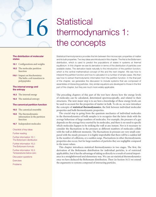
<strong>Statistical</strong> <strong><strong>the</strong>rmodynamics</strong> provides <strong>the</strong> link between <strong>the</strong> microscopic properties of matter<br />
and its bulk properties. Two key ideas are introduced in this chapter. The first is <strong>the</strong> Boltzmann<br />
distribution, which is used to predict <strong>the</strong> populations of states in systems at <strong>the</strong>rmal<br />
equilibrium. In this chapter we see its derivation in terms of <strong>the</strong> distribution of particles over<br />
available states. The derivation leads naturally to <strong>the</strong> introduction of <strong>the</strong> partition function,<br />
which is <strong>the</strong> central ma<strong>the</strong>matical concept of this and <strong>the</strong> next chapter. We see how to<br />
interpret <strong>the</strong> partition function and how to calculate it in a number of simple cases. We <strong>the</strong>n<br />
see how to extract <strong>the</strong>rmodynamic information from <strong>the</strong> partition function. In <strong>the</strong> final part<br />
of <strong>the</strong> chapter, we generalize <strong>the</strong> discussion to include systems that are composed of<br />
assemblies of interacting particles. Very similar equations are developed to those in <strong>the</strong> first<br />
part of <strong>the</strong> chapter, but <strong>the</strong>y are much more widely applicable.<br />
The preceding chapters of this part of <strong>the</strong> text have shown how <strong>the</strong> energy levels<br />
of molecules can be calculated, determined spectroscopically, and related to <strong>the</strong>ir<br />
structures. The next major step is to see how a knowledge of <strong>the</strong>se energy levels can<br />
be used to account for <strong>the</strong> properties of matter in bulk. To do so, we now introduce<br />
<strong>the</strong> <strong>concepts</strong> of statistical <strong><strong>the</strong>rmodynamics</strong>, <strong>the</strong> link between individual molecular<br />
properties and bulk <strong>the</strong>rmodynamic properties.<br />
The crucial step in going from <strong>the</strong> quantum mechanics of individual molecules<br />
to <strong>the</strong> <strong><strong>the</strong>rmodynamics</strong> of bulk samples is to recognize that <strong>the</strong> latter deals with <strong>the</strong><br />
average behaviour of large numbers of molecules. For example, <strong>the</strong> pressure of a gas<br />
depends on <strong>the</strong> average force exerted by its molecules, and <strong>the</strong>re is no need to specify<br />
which molecules happen to be striking <strong>the</strong> wall at any instant. Nor is it necessary to<br />
consider <strong>the</strong> fluctuations in <strong>the</strong> pressure as different numbers of molecules collide<br />
with <strong>the</strong> wall at different moments. The fluctuations in pressure are very small compared<br />
with <strong>the</strong> steady pressure: it is highly improbable that <strong>the</strong>re will be a sudden lull<br />
in <strong>the</strong> number of collisions, or a sudden surge. Fluctuations in o<strong>the</strong>r <strong>the</strong>rmodynamic<br />
properties also occur, but for large numbers of particles <strong>the</strong>y are negligible compared<br />
to <strong>the</strong> mean values.<br />
This chapter introduces statistical <strong><strong>the</strong>rmodynamics</strong> in two stages. The first, <strong>the</strong><br />
derivation of <strong>the</strong> Boltzmann distribution for individual particles, is of restricted<br />
applicability, but it has <strong>the</strong> advantage of taking us directly to a result of central importance<br />
in a straightforward and elementary way. We can use statistical <strong><strong>the</strong>rmodynamics</strong><br />
once we have deduced <strong>the</strong> Boltzmann distribution. Then (in Section 16.5) we extend<br />
<strong>the</strong> arguments to systems composed of interacting particles.
PC8eC16 1/26/06 14:34 Page 561<br />
16.1 CONFIGURATIONS AND WEIGHTS 561<br />
The distribution of molecular states<br />
We consider a closed system composed of N molecules. Although <strong>the</strong> total energy is<br />
constant at E, it is not possible to be definite about how that energy is shared between<br />
<strong>the</strong> molecules. Collisions result in <strong>the</strong> ceaseless redistribution of energy not only<br />
between <strong>the</strong> molecules but also among <strong>the</strong>ir different modes of motion. The closest<br />
we can come to a description of <strong>the</strong> distribution of energy is to report <strong>the</strong> population<br />
of a state, <strong>the</strong> average number of molecules that occupy it, and to say that on average<br />
<strong>the</strong>re are n i molecules in a state of energy ε i . The populations of <strong>the</strong> states remain<br />
almost constant, but <strong>the</strong> precise identities of <strong>the</strong> molecules in each state may change<br />
at every collision.<br />
The problem we address in this section is <strong>the</strong> calculation of <strong>the</strong> populations of states<br />
for any type of molecule in any mode of motion at any temperature. The only restriction<br />
is that <strong>the</strong> molecules should be independent, in <strong>the</strong> sense that <strong>the</strong> total energy<br />
of <strong>the</strong> system is a sum of <strong>the</strong>ir individual energies. We are discounting (at this stage)<br />
<strong>the</strong> possibility that in a real system a contribution to <strong>the</strong> total energy may arise from<br />
interactions between molecules. We also adopt <strong>the</strong> principle of equal a priori probabilities,<br />
<strong>the</strong> assumption that all possibilities for <strong>the</strong> distribution of energy are equally<br />
probable. A priori means in this context loosely ‘as far as one knows’. We have no reason<br />
to presume o<strong>the</strong>rwise than that, for a collection of molecules at <strong>the</strong>rmal equilibrium,<br />
vibrational states of a certain energy, for instance, are as likely to be populated as<br />
rotational states of <strong>the</strong> same energy.<br />
One very important conclusion that will emerge from <strong>the</strong> following analysis is that<br />
<strong>the</strong> populations of states depend on a single parameter, <strong>the</strong> ‘temperature’. That is, statistical<br />
<strong><strong>the</strong>rmodynamics</strong> provides a molecular justification for <strong>the</strong> concept of temperature<br />
and some insight into this crucially important quantity.<br />
16.1 Configurations and weights<br />
Any individual molecule may exist in states with energies ε 0 , ε 1 ,....We shall always<br />
take ε 0 , <strong>the</strong> lowest state, as <strong>the</strong> zero of energy (ε 0 = 0), and measure all o<strong>the</strong>r energies<br />
relative to that state. To obtain <strong>the</strong> actual internal energy, U, we may have to add a<br />
constant to <strong>the</strong> calculated energy of <strong>the</strong> system. For example, if we are considering <strong>the</strong><br />
vibrational contribution to <strong>the</strong> internal energy, <strong>the</strong>n we must add <strong>the</strong> total zero-point<br />
energy of any oscillators in <strong>the</strong> sample.<br />
(a) Instantaneous configurations<br />
At any instant <strong>the</strong>re will be n 0 molecules in <strong>the</strong> state with energy ε 0 , n 1 with ε 1 , and so<br />
on. The specification of <strong>the</strong> set of populations n 0 , n 1 ,...in <strong>the</strong> form {n 0 , n 1 ,...} is a<br />
statement of <strong>the</strong> instantaneous configuration of <strong>the</strong> system. The instantaneous<br />
configuration fluctuates with time because <strong>the</strong> populations change. We can picture a<br />
large number of different instantaneous configurations. One, for example, might be<br />
{N,0,0, ...}, corresponding to every molecule being in its ground state. Ano<strong>the</strong>r<br />
might be {N − 2,2,0,0, ...}, in which two molecules are in <strong>the</strong> first excited state.<br />
The latter configuration is intrinsically more likely to be found than <strong>the</strong> former<br />
because it can be achieved in more ways: {N,0,0, ...} can be achieved in only one<br />
way, but {N − 2,2,0, ...} can be achieved in – 1 2<br />
N(N − 1) different ways (Fig. 16.1; see<br />
Justification 16.1). At this stage in <strong>the</strong> argument, we are ignoring <strong>the</strong> requirement<br />
that <strong>the</strong> total energy of <strong>the</strong> system should be constant (<strong>the</strong> second configuration has<br />
a higher energy than <strong>the</strong> first). The constraint of total energy is imposed later in this<br />
section.<br />
Fig. 16.1 Whereas a configuration<br />
{5,0,0, ...} can be achieved in only one<br />
way, a configuration {3,2,0, ...} can be<br />
achieved in <strong>the</strong> ten different ways shown<br />
here, where <strong>the</strong> tinted blocks represent<br />
different molecules.
PC8eC16 1/26/06 14:34 Page 562<br />
562 16 STATISTICAL THERMODYNAMICS 1: THE CONCEPTS<br />
Fig. 16.2 The 18 molecules shown here can<br />
be distributed into four receptacles<br />
(distinguished by <strong>the</strong> three vertical lines)<br />
in 18! different ways. However, 3! of <strong>the</strong><br />
selections that put three molecules in <strong>the</strong><br />
first receptacle are equivalent, 6! that put<br />
six molecules into <strong>the</strong> second receptacle are<br />
equivalent, and so on. Hence <strong>the</strong> number<br />
of distinguishable arrangements is<br />
18!/3!6!5!4!.<br />
Comment 16.1<br />
More formally, W is called <strong>the</strong><br />
multinomial coefficient (see Appendix 2).<br />
In eqn 16.1, x!, x factorial, denotes<br />
x(x − 1)(x − 2)...1, and by definition<br />
0! = 1.<br />
N = 18<br />
3! 6! 5! 4!<br />
If, as a result of collisions, <strong>the</strong> system were to fluctuate between <strong>the</strong> configurations<br />
{N,0,0, ...} and {N − 2,2,0, ...}, it would almost always be found in <strong>the</strong> second,<br />
more likely state (especially if N were large). In o<strong>the</strong>r words, a system free to switch<br />
between <strong>the</strong> two configurations would show properties characteristic almost exclusively<br />
of <strong>the</strong> second configuration. A general configuration {n 0 ,n 1 ,...} can be achieved<br />
in W different ways, where W is called <strong>the</strong> weight of <strong>the</strong> configuration. The weight of<br />
<strong>the</strong> configuration {n 0 ,n 1 ,...} is given by <strong>the</strong> expression<br />
N!<br />
W = (16.1)<br />
n 0 !n 1 !n 2 !...<br />
Equation 16.1 is a generalization of <strong>the</strong> formula W = – 1 2<br />
N(N − 1), and reduces to it for<br />
<strong>the</strong> configuration {N − 2,2,0, ...}.<br />
Justification 16.1 The weight of a configuration<br />
First, consider <strong>the</strong> weight of <strong>the</strong> configuration {N − 2,2,0,0, ...}. One candidate for<br />
promotion to an upper state can be selected in N ways. There are N − 1 candidates<br />
for <strong>the</strong> second choice, so <strong>the</strong> total number of choices is N(N − 1). However, we<br />
should not distinguish <strong>the</strong> choice (Jack, Jill) from <strong>the</strong> choice (Jill, Jack) because <strong>the</strong>y<br />
lead to <strong>the</strong> same configurations. Therefore, only half <strong>the</strong> choices lead to distinguishable<br />
configurations, and <strong>the</strong> total number of distinguishable choices is 1 – 2 N(N − 1).<br />
Now we generalize this remark. Consider <strong>the</strong> number of ways of distributing<br />
N balls into bins. The first ball can be selected in N different ways, <strong>the</strong> next ball<br />
in N − 1 different ways for <strong>the</strong> balls remaining, and so on. Therefore, <strong>the</strong>re are<br />
N(N − 1)...1 = N! ways of selecting <strong>the</strong> balls for distribution over <strong>the</strong> bins.<br />
However, if <strong>the</strong>re are n 0 balls in <strong>the</strong> bin labelled ε 0 , <strong>the</strong>re would be n 0 ! different ways<br />
in which <strong>the</strong> same balls could have been chosen (Fig. 16.2). Similarly, <strong>the</strong>re are<br />
n 1 ! ways in which <strong>the</strong> n 1 balls in <strong>the</strong> bin labelled ε 1 can be chosen, and so on.<br />
Therefore, <strong>the</strong> total number of distinguishable ways of distributing <strong>the</strong> balls so that<br />
<strong>the</strong>re are n 0 in bin ε 0 , n 1 in bin ε 1 , etc. regardless of <strong>the</strong> order in which <strong>the</strong> balls were<br />
chosen is N!/n 0 !n 1 !..., which is <strong>the</strong> content of eqn 16.1.<br />
Illustration 16.1 Calculating <strong>the</strong> weight of a distribution<br />
To calculate <strong>the</strong> number of ways of distributing 20 identical objects with <strong>the</strong><br />
arrangement 1, 0, 3, 5, 10, 1, we note that <strong>the</strong> configuration is {1,0,3,5,10,1} with<br />
N = 20; <strong>the</strong>refore <strong>the</strong> weight is<br />
20!<br />
W = = 9.31 × 10 8<br />
1!0!3!5!10!1!<br />
Self-test 16.1 Calculate <strong>the</strong> weight of <strong>the</strong> configuration in which 20 objects are<br />
distributed in <strong>the</strong> arrangement 0, 1, 5, 0, 8, 0, 3, 2, 0, 1. [4.19 × 10 10 ]
PC8eC16 1/26/06 14:34 Page 563<br />
16.1 CONFIGURATIONS AND WEIGHTS 563<br />
It will turn out to be more convenient to deal with <strong>the</strong> natural logarithm of <strong>the</strong><br />
weight, ln W, ra<strong>the</strong>r than with <strong>the</strong> weight itself. We shall <strong>the</strong>refore need <strong>the</strong> expression<br />
N!<br />
ln W = ln = ln N! − ln(n 0 !n 1 !n 2 ! · · · )<br />
n 0 !n 1 !n 2 !...<br />
= ln N! − (ln n 0 ! + ln n 1 ! + ln n 2 ! + · · · )<br />
= ln N! − ∑ln n i !<br />
i<br />
where in <strong>the</strong> first line we have used ln(x/y) = ln x − ln y and in <strong>the</strong> second ln xy = ln x<br />
+ ln y. One reason for introducing ln W is that it is easier to make approximations. In<br />
particular, we can simplify <strong>the</strong> factorials by using Stirling’s approximation in <strong>the</strong> form<br />
ln x! ≈ x ln x − x (16.2)<br />
Then <strong>the</strong> approximate expression for <strong>the</strong> weight is<br />
ln W = (N ln N − N) − ∑<br />
i<br />
(n i ln n i − n i ) = N ln N − ∑n i ln n i (16.3)<br />
i<br />
The final form of eqn 16.3 is derived by noting that <strong>the</strong> sum of n i is equal to N, so <strong>the</strong><br />
second and fourth terms in <strong>the</strong> second expression cancel.<br />
(b) The Boltzmann distribution<br />
We have seen that <strong>the</strong> configuration {N − 2,2,0, ...} dominates {N,0,0, ...}, and it<br />
should be easy to believe that <strong>the</strong>re may be o<strong>the</strong>r configurations that have a much<br />
greater weight than both. We shall see, in fact, that <strong>the</strong>re is a configuration with so<br />
great a weight that it overwhelms all <strong>the</strong> rest in importance to such an extent that <strong>the</strong><br />
system will almost always be found in it. The properties of <strong>the</strong> system will <strong>the</strong>refore be<br />
characteristic of that particular dominating configuration. This dominating configuration<br />
can be found by looking for <strong>the</strong> values of n i that lead to a maximum value of W.<br />
Because W is a function of all <strong>the</strong> n i , we can do this search by varying <strong>the</strong> n i and looking<br />
for <strong>the</strong> values that correspond to dW = 0 (just as in <strong>the</strong> search for <strong>the</strong> maximum of<br />
any function), or equivalently a maximum value of ln W. However, <strong>the</strong>re are two<br />
difficulties with this procedure.<br />
The first difficulty is that <strong>the</strong> only permitted configurations are those corresponding<br />
to <strong>the</strong> specified, constant, total energy of <strong>the</strong> system. This requirement rules out<br />
many configurations; {N,0,0, ...} and {N − 2,2,0, ...}, for instance, have different<br />
energies, so both cannot occur in <strong>the</strong> same isolated system. It follows that, in looking<br />
for <strong>the</strong> configuration with <strong>the</strong> greatest weight, we must ensure that <strong>the</strong> configuration<br />
also satisfies <strong>the</strong> condition<br />
Constant total energy: ∑n i ε i = E (16.4)<br />
i<br />
where E is <strong>the</strong> total energy of <strong>the</strong> system.<br />
The second constraint is that, because <strong>the</strong> total number of molecules present is<br />
also fixed (at N), we cannot arbitrarily vary all <strong>the</strong> populations simultaneously. Thus,<br />
increasing <strong>the</strong> population of one state by 1 demands that <strong>the</strong> population of ano<strong>the</strong>r<br />
state must be reduced by 1. Therefore, <strong>the</strong> search for <strong>the</strong> maximum value of W is also<br />
subject to <strong>the</strong> condition<br />
Constant total number of molecules: ∑n i = N (16.5)<br />
i<br />
We show in Fur<strong>the</strong>r information 16.1 that <strong>the</strong> populations in <strong>the</strong> configuration of<br />
greatest weight, subject to <strong>the</strong> two constraints in eqns 16.4 and 16.5, depend on <strong>the</strong><br />
energy of <strong>the</strong> state according to <strong>the</strong> Boltzmann distribution:<br />
Comment 16.2<br />
A more accurate form of Stirling’s<br />
approximation is<br />
x! ≈ (2π) 1/2 x x+ – 2e 1 −x<br />
and is in error by less than 1 per cent<br />
when x is greater than about 10. We deal<br />
with far larger values of x, and <strong>the</strong><br />
simplified version in eqn 16.2 is<br />
adequate.
PC8eC16 1/26/06 14:34 Page 564<br />
564 16 STATISTICAL THERMODYNAMICS 1: THE CONCEPTS<br />
n i<br />
N<br />
e −βε i<br />
∑ e −βε i<br />
i<br />
= (16.6a)<br />
where ε 0 ≤ ε 1 ≤ ε 2 ....Equation 16.6a is <strong>the</strong> justification of <strong>the</strong> remark that a single<br />
parameter, here denoted β, determines <strong>the</strong> most probable populations of <strong>the</strong> states of<br />
<strong>the</strong> system. We shall see in Section 16.3b that<br />
1<br />
β =<br />
(16.6b)<br />
kT<br />
where T is <strong>the</strong> <strong>the</strong>rmodynamic temperature and k is Boltzmann’s constant. In o<strong>the</strong>r<br />
words, <strong>the</strong> <strong>the</strong>rmodynamic temperature is <strong>the</strong> unique parameter that governs <strong>the</strong> most<br />
probable populations of states of a system at <strong>the</strong>rmal equilibrium. In Fur<strong>the</strong>r information<br />
16.3, moreover, we see that β is a more natural measure of temperature than T itself.<br />
16.2 The molecular partition function<br />
From now on we write <strong>the</strong> Boltzmann distribution as<br />
e −βε i<br />
p i = (16.7)<br />
q<br />
where p i is <strong>the</strong> fraction of molecules in <strong>the</strong> state i, p i = n i /N, and q is <strong>the</strong> molecular<br />
partition function:<br />
q = ∑ e −βε i<br />
[16.8]<br />
i<br />
The sum in q is sometimes expressed slightly differently. It may happen that several states<br />
have <strong>the</strong> same energy, and so give <strong>the</strong> same contribution to <strong>the</strong> sum. If, for example,<br />
g i states have <strong>the</strong> same energy ε i (so <strong>the</strong> level is g i -fold degenerate), we could write<br />
q = ∑ g i e −βε i<br />
(16.9)<br />
levels i<br />
where <strong>the</strong> sum is now over energy levels (sets of states with <strong>the</strong> same energy), not<br />
individual states.<br />
Example 16.1 Writing a partition function<br />
Write an expression for <strong>the</strong> partition function of a linear molecule (such as HCl)<br />
treated as a rigid rotor.<br />
Method To use eqn 16.9 we need to know (a) <strong>the</strong> energies of <strong>the</strong> levels, (b) <strong>the</strong><br />
degeneracies, <strong>the</strong> number of states that belong to each level. Whenever calculating<br />
a partition function, <strong>the</strong> energies of <strong>the</strong> levels are expressed relative to 0 for <strong>the</strong> state<br />
of lowest energy. The energy levels of a rigid linear rotor were derived in Section 13.5c.<br />
Answer From eqn 13.31, <strong>the</strong> energy levels of a linear rotor are hcBJ(J + 1), with<br />
J = 0, 1, 2,....The state of lowest energy has zero energy, so no adjustment need<br />
be made to <strong>the</strong> energies given by this expression. Each level consists of 2J + 1<br />
degenerate states. Therefore,<br />
q =<br />
∞<br />
∑<br />
J=0<br />
g J<br />
5<br />
6<br />
7<br />
5<br />
67<br />
ε J<br />
(2J + 1)e −βhcBJ(J+1)<br />
The sum can be evaluated numerically by supplying <strong>the</strong> value of B (from spectroscopy<br />
or calculation) and <strong>the</strong> temperature. For reasons explained in Section 17.2b,
PC8eC16 1/27/06 22:03 Page 565<br />
16.2 THE MOLECULAR PARTITION FUNCTION 565<br />
this expression applies only to unsymmetrical linear rotors (for instance, HCl,<br />
not CO 2 ).<br />
Self-test 16.2 Write <strong>the</strong> partition function for a two-level system, <strong>the</strong> lower state<br />
(at energy 0) being nondegenerate, and <strong>the</strong> upper state (at an energy ε) doubly<br />
degenerate. [q = 1 + 2e −βε ]<br />
e<br />
(a) An interpretation of <strong>the</strong> partition function<br />
Some insight into <strong>the</strong> significance of a partition function can be obtained by considering<br />
how q depends on <strong>the</strong> temperature. When T is close to zero, <strong>the</strong> parameter<br />
β = 1/kT is close to infinity. Then every term except one in <strong>the</strong> sum defining q is zero<br />
because each one has <strong>the</strong> form e −x with x →∞. The exception is <strong>the</strong> term with ε 0 ≡ 0<br />
(or <strong>the</strong> g 0 terms at zero energy if <strong>the</strong> ground state is g 0 -fold degenerate), because <strong>the</strong>n<br />
ε 0 /kT ≡ 0 whatever <strong>the</strong> temperature, including zero. As <strong>the</strong>re is only one surviving<br />
term when T = 0, and its value is g 0 , it follows that<br />
lim q = g 0 (16.10)<br />
T→0<br />
That is, at T = 0, <strong>the</strong> partition function is equal to <strong>the</strong> degeneracy of <strong>the</strong> ground state.<br />
Now consider <strong>the</strong> case when T is so high that for each term in <strong>the</strong> sum ε j /kT ≈ 0.<br />
Because e −x = 1 when x = 0, each term in <strong>the</strong> sum now contributes 1. It follows that <strong>the</strong><br />
sum is equal to <strong>the</strong> number of molecular states, which in general is infinite:<br />
lim q =∞ (16.11)<br />
T→∞<br />
In some idealized cases, <strong>the</strong> molecule may have only a finite number of states; <strong>the</strong>n <strong>the</strong><br />
upper limit of q is equal to <strong>the</strong> number of states. For example, if we were considering<br />
only <strong>the</strong> spin energy levels of a radical in a magnetic field, <strong>the</strong>n <strong>the</strong>re would be only<br />
two states (m s =± – 1 2<br />
). The partition function for such a system can <strong>the</strong>refore be<br />
expected to rise towards 2 as T is increased towards infinity.<br />
We see that <strong>the</strong> molecular partition function gives an indication of <strong>the</strong> number of states<br />
that are <strong>the</strong>rmally accessible to a molecule at <strong>the</strong> temperature of <strong>the</strong> system. At T = 0, only<br />
<strong>the</strong> ground level is accessible and q = g 0 . At very high temperatures, virtually all states<br />
are accessible, and q is correspondingly large.<br />
Example 16.2 Evaluating <strong>the</strong> partition function for a uniform ladder of energy levels<br />
Evaluate <strong>the</strong> partition function for a molecule with an infinite number of equally<br />
spaced nondegenerate energy levels (Fig. 16.3). These levels can be thought of as <strong>the</strong><br />
vibrational energy levels of a diatomic molecule in <strong>the</strong> harmonic approximation.<br />
Method We expect <strong>the</strong> partition function to increase from 1 at T = 0 and approach<br />
infinity as T to ∞. To evaluate eqn 16.8 explicitly, note that<br />
1<br />
1 + x + x 2 + ···=<br />
1 − x<br />
Answer If <strong>the</strong> separation of neighbouring levels is ε, <strong>the</strong> partition function is<br />
1<br />
q = 1 + e −βε + e −2βε + ···= 1 + e −βε + (e −βε ) 2 + ···=<br />
1 − e −βε<br />
This expression is plotted in Fig. 16.4: notice that, as anticipated, q rises from 1 to<br />
infinity as <strong>the</strong> temperature is raised.<br />
3e<br />
2e<br />
e<br />
0<br />
Fig. 16.3 The equally spaced infinite array of<br />
energy levels used in <strong>the</strong> calculation of <strong>the</strong><br />
partition function. A harmonic oscillator<br />
has <strong>the</strong> same spectrum of levels.<br />
Comment 16.3<br />
The sum of <strong>the</strong> infinite series S = 1 + x +<br />
x 2 + · · · is obtained by multiplying both<br />
sides by x, which gives xS = x + x 2 + x 3<br />
+ · · · = S − 1 and hence S = 1/(1 − x).<br />
10<br />
q<br />
5<br />
0<br />
0 5 10<br />
kT/<br />
Fig. 16.4 The partition function for <strong>the</strong><br />
system shown in Fig.16.3 (a harmonic<br />
oscillator) as a function of temperature.<br />
Exploration Plot <strong>the</strong> partition<br />
function of a harmonic oscillator<br />
against temperature for several values of<br />
<strong>the</strong> energy separation ε. How does q vary<br />
with temperature when T is high, in <strong>the</strong><br />
sense that kT >> ε (or βε
PC8eC16 1/26/06 14:34 Page 566<br />
566 16 STATISTICAL THERMODYNAMICS 1: THE CONCEPTS<br />
1.4<br />
2<br />
q<br />
q<br />
1.2<br />
1.5<br />
1<br />
0 0.5 1<br />
kT/ <br />
1 0 5 10<br />
kT/ <br />
Low<br />
temperature<br />
High<br />
temperature<br />
Fig. 16.5 The partition function for a two-level system as a function of temperature. The two<br />
graphs differ in <strong>the</strong> scale of <strong>the</strong> temperature axis to show <strong>the</strong> approach to 1 as T → 0 and <strong>the</strong><br />
slow approach to 2 as T →∞.<br />
Exploration Consider a three-level system with levels 0, ε, and 2ε. Plot <strong>the</strong> partition<br />
function against kT/ε.<br />
Self-test 16.3 Find and plot an expression for <strong>the</strong> partition function of a system<br />
with one state at zero energy and ano<strong>the</strong>r state at <strong>the</strong> energy ε.<br />
[q = 1 + e −βε , Fig. 16.5]<br />
It follows from eqn 16.8 and <strong>the</strong> expression for q derived in Example 16.2 for a uniform<br />
ladder of states of spacing ε,<br />
1<br />
q = (16.12)<br />
1 − e −βε<br />
that <strong>the</strong> fraction of molecules in <strong>the</strong> state with energy ε i is<br />
<br />
3.0 1.0 0.7 0.3<br />
q: 1.05 1.58 1.99 3.86<br />
Fig. 16.6 The populations of <strong>the</strong> energy<br />
levels of <strong>the</strong> system shown in Fig.16.3<br />
at different temperatures, and <strong>the</strong><br />
corresponding values of <strong>the</strong> partition<br />
function calculated in Example 16.2.<br />
Note that β = 1/kT.<br />
Exploration To visualize <strong>the</strong> content<br />
of Fig. 16.6 in a different way, plot<br />
<strong>the</strong> functions p 0 , p 1 , p 2 , and p 3 against kT/ε.<br />
e −βε i<br />
p i = =(1 − e −βε )e −βε i<br />
(16.13)<br />
q<br />
Figure 16.6 shows how p i varies with temperature. At very low temperatures, where q<br />
is close to 1, only <strong>the</strong> lowest state is significantly populated. As <strong>the</strong> temperature is<br />
raised, <strong>the</strong> population breaks out of <strong>the</strong> lowest state, and <strong>the</strong> upper states become<br />
progressively more highly populated. At <strong>the</strong> same time, <strong>the</strong> partition function rises<br />
from 1 and its value gives an indication of <strong>the</strong> range of states populated. The name<br />
‘partition function’ reflects <strong>the</strong> sense in which q measures how <strong>the</strong> total number of<br />
molecules is distributed—partitioned—over <strong>the</strong> available states.<br />
The corresponding expressions for a two-level system derived in Self-test 16.3 are<br />
1<br />
e −βε<br />
p 0 = p 1 = (16.14)<br />
1 + e −βε 1 + e −βε<br />
These functions are plotted in Fig. 16.7. Notice how <strong>the</strong> populations tend towards<br />
equality (p 0 = – 1 2<br />
, p 1 = – 1 2<br />
) as T →∞. A common error is to suppose that all <strong>the</strong> molecules<br />
in <strong>the</strong> system will be found in <strong>the</strong> upper energy state when T =∞; however, we see
PC8eC16 1/26/06 14:34 Page 567<br />
16.2 THE MOLECULAR PARTITION FUNCTION 567<br />
1<br />
1<br />
p p 0<br />
p<br />
p 0<br />
0.5<br />
0.5<br />
p 1<br />
p 1<br />
0<br />
0<br />
0 0.5<br />
kT/ <br />
1<br />
0 5 10<br />
kT/ <br />
Fig. 16.7 The fraction of populations of <strong>the</strong> two states of a two-level system as a function of<br />
temperature (eqn 16.14). Note that, as <strong>the</strong> temperature approaches infinity, <strong>the</strong> populations<br />
of <strong>the</strong> two states become equal (and <strong>the</strong> fractions both approach 0.5).<br />
Exploration Consider a three-level system with levels 0, ε, and 2ε. Plot <strong>the</strong> functions p 0 ,<br />
p 1 , and p 2 against kT/ε.<br />
from eqn 16.14 that, as T →∞, <strong>the</strong> populations of states become equal. The same<br />
conclusion is true of multi-level systems too: as T →∞, all states become equally<br />
populated.<br />
Example 16.3 Using <strong>the</strong> partition function to calculate a population<br />
Calculate <strong>the</strong> proportion of I 2 molecules in <strong>the</strong>ir ground, first excited, and second<br />
excited vibrational states at 25°C. The vibrational wavenumber is 214.6 cm −1 .<br />
Method Vibrational energy levels have a constant separation (in <strong>the</strong> harmonic<br />
approximation, Section 13.9), so <strong>the</strong> partition function is given by eqn 16.12 and<br />
<strong>the</strong> populations by eqn 16.13. To use <strong>the</strong> latter equation, we identify <strong>the</strong> index<br />
i with <strong>the</strong> quantum number v, and calculate p v for v = 0, 1, and 2. At 298.15 K,<br />
kT/hc = 207.226 cm −1 .<br />
Answer First, we note that<br />
hc# 214.6 cm −1<br />
βε = = =1.036<br />
kT 207.226 cm −1<br />
Then it follows from eqn 16.13 that <strong>the</strong> populations are<br />
p v = (1 − e −βε )e −vβε = 0.645e −1.036v<br />
Therefore, p 0 = 0.645, p 1 = 0.229, p 2 = 0.081. The I-I bond is not stiff and <strong>the</strong> atoms<br />
are heavy: as a result, <strong>the</strong> vibrational energy separations are small and at room<br />
temperature several vibrational levels are significantly populated. The value of <strong>the</strong><br />
partition function, q = 1.55, reflects this small but significant spread of populations.<br />
Self-test 16.4 At what temperature would <strong>the</strong> v = 1 level of I 2 have (a) half <strong>the</strong> population<br />
of <strong>the</strong> ground state, (b) <strong>the</strong> same population as <strong>the</strong> ground state<br />
[(a) 445 K, (b) infinite]
PC8eC16 1/26/06 14:34 Page 568<br />
568 16 STATISTICAL THERMODYNAMICS 1: THE CONCEPTS<br />
Entropy, S<br />
0<br />
C<br />
Magnetic<br />
field off<br />
Magnetic<br />
field on<br />
Temperature, T<br />
Fig. 16.8 The technique of adiabatic<br />
demagnetization is used to attain very low<br />
temperatures. The upper curve shows that<br />
variation of <strong>the</strong> entropy of a paramagnetic<br />
system in <strong>the</strong> absence of an applied field.<br />
The lower curve shows that variation in<br />
entropy when a field is applied and has<br />
made <strong>the</strong> electron magnets more orderly.<br />
The iso<strong>the</strong>rmal magnetization step is from<br />
A to B; <strong>the</strong> adiabatic demagnetization step<br />
(at constant entropy) is from B to C.<br />
A<br />
B<br />
It follows from our discussion of <strong>the</strong> partition function that to reach low temperatures<br />
it is necessary to devise strategies that populate <strong>the</strong> low energy levels of a system<br />
at <strong>the</strong> expense of high energy levels. Common methods used to reach very low<br />
temperatures include optical trapping and adiabatic demagnetization. In optical<br />
trapping, atoms in <strong>the</strong> gas phase are cooled by inelastic collisions with photons from<br />
intense laser beams, which act as walls of a very small container. Adiabatic demagnetization<br />
is based on <strong>the</strong> fact that, in <strong>the</strong> absence of a magnetic field, <strong>the</strong> unpaired electrons<br />
of a paramagnetic material are orientated at random, but in <strong>the</strong> presence of a<br />
magnetic field <strong>the</strong>re are more β spins (m s =− 1 – 2<br />
) than α spins (m s =+ 1 – 2<br />
). In <strong>the</strong>rmodynamic<br />
terms, <strong>the</strong> application of a magnetic field lowers <strong>the</strong> entropy of a sample and,<br />
at a given temperature, <strong>the</strong> entropy of a sample is lower when <strong>the</strong> field is on than when<br />
it is off. Even lower temperatures can be reached if nuclear spins (which also behave<br />
like small magnets) are used instead of electron spins in <strong>the</strong> technique of adiabatic<br />
nuclear demagnetization, which has been used to cool a sample of silver to about<br />
280 pK. In certain circumstances it is possible to achieve negative temperatures, and<br />
<strong>the</strong> equations derived later in this chapter can be extended to T < 0 with interesting<br />
consequences (see Fur<strong>the</strong>r information 16.3).<br />
Illustration 16.2 Cooling a sample by adiabatic demagnetization<br />
Consider <strong>the</strong> situation summarized by Fig. 16.8. A sample of paramagnetic<br />
material, such as a d- or f-metal complex with several unpaired electrons, is cooled<br />
to about 1 K by using helium. The sample is <strong>the</strong>n exposed to a strong magnetic<br />
field while it is surrounded by helium, which provides <strong>the</strong>rmal contact with <strong>the</strong><br />
cold reservoir. This magnetization step is iso<strong>the</strong>rmal, and energy leaves <strong>the</strong> system<br />
as heat while <strong>the</strong> electron spins adopt <strong>the</strong> lower energy state (AB in <strong>the</strong> illustration).<br />
Thermal contact between <strong>the</strong> sample and <strong>the</strong> surroundings is now broken<br />
by pumping away <strong>the</strong> helium and <strong>the</strong> magnetic field is reduced to zero. This<br />
step is adiabatic and effectively reversible, so <strong>the</strong> state of <strong>the</strong> sample changes from<br />
B to C. At <strong>the</strong> end of this step <strong>the</strong> sample is <strong>the</strong> same as it was at A except that it<br />
now has a lower entropy. That lower entropy in <strong>the</strong> absence of a magnetic field corresponds<br />
to a lower temperature. That is, adiabatic demagnetization has cooled<br />
<strong>the</strong> sample.<br />
(b) Approximations and factorizations<br />
In general, exact analytical expressions for partition functions cannot be obtained.<br />
However, closed approximate expressions can often be found and prove to be very<br />
important in a number of chemical and biochemical applications (Impact 16.1). For<br />
instance, <strong>the</strong> expression for <strong>the</strong> partition function for a particle of mass m free to move<br />
in a one-dimensional container of length X can be evaluated by making use of <strong>the</strong> fact<br />
that <strong>the</strong> separation of energy levels is very small and that large numbers of states are<br />
accessible at normal temperatures. As shown in <strong>the</strong> Justification below, in this case<br />
1/2<br />
A 2πmD<br />
q X = X (16.15)<br />
C h 2 β F<br />
This expression shows that <strong>the</strong> partition function for translational motion increases<br />
with <strong>the</strong> length of <strong>the</strong> box and <strong>the</strong> mass of <strong>the</strong> particle, for in each case <strong>the</strong> separation<br />
of <strong>the</strong> energy levels becomes smaller and more levels become <strong>the</strong>rmally accessible. For<br />
a given mass and length of <strong>the</strong> box, <strong>the</strong> partition function also increases with increasing<br />
temperature (decreasing β), because more states become accessible.
PC8eC16 1/26/06 14:34 Page 569<br />
16.2 THE MOLECULAR PARTITION FUNCTION 569<br />
Justification 16.2 The partition function for a particle in a one-dimensional box<br />
The energy levels of a molecule of mass m in a container of length X are given by<br />
eqn 9.4a with L = X:<br />
n 2 h 2<br />
E n = n = 1, 2,...<br />
8mX 2<br />
The lowest level (n = 1) has energy h 2 /8mX 2 , so <strong>the</strong> energies relative to that level are<br />
ε n = (n 2 − 1)ε ε= h 2 /8mX 2<br />
The sum to evaluate is <strong>the</strong>refore<br />
q X =<br />
∞<br />
∑ e −(n2 −1)βε<br />
n=1<br />
The translational energy levels are very close toge<strong>the</strong>r in a container <strong>the</strong> size of a typical<br />
laboratory vessel; <strong>the</strong>refore, <strong>the</strong> sum can be approximated by an integral:<br />
∞<br />
∞<br />
q X = <br />
e −(n2−1)βε dn ≈ <br />
e −n2βε dn<br />
1<br />
0<br />
The extension of <strong>the</strong> lower limit to n = 0 and <strong>the</strong> replacement of n 2 − 1 by n 2 introduces<br />
negligible error but turns <strong>the</strong> integral into standard form. We make <strong>the</strong><br />
substitution x 2 = n 2 βε, implying dn = dx/(βε) 1/2 , and <strong>the</strong>refore that<br />
A 1 D<br />
q X = B E<br />
C βε F<br />
1/2<br />
∞ 0<br />
π 1/2 /2<br />
5<br />
6<br />
7<br />
A 1 D<br />
e −x2 dx = B E<br />
C βε F<br />
1/2<br />
A D A 2πmD<br />
B E = B E<br />
C 2 F C h 2 β F<br />
π 1/2<br />
1/2<br />
X<br />
Ano<strong>the</strong>r useful feature of partition functions is used to derive expressions when <strong>the</strong><br />
energy of a molecule arises from several different, independent sources: if <strong>the</strong> energy<br />
is a sum of contributions from independent modes of motion, <strong>the</strong>n <strong>the</strong> partition<br />
function is a product of partition functions for each mode of motion. For instance,<br />
suppose <strong>the</strong> molecule we are considering is free to move in three dimensions. We take<br />
<strong>the</strong> length of <strong>the</strong> container in <strong>the</strong> y-direction to be Y and that in <strong>the</strong> z-direction to be<br />
Z. The total energy of a molecule ε is <strong>the</strong> sum of its translational energies in all three<br />
directions:<br />
ε n1 n 2 n 3<br />
= ε (X) n1<br />
+ ε (Y) (Z)<br />
n2<br />
+ ε n3<br />
(16.16)<br />
where n 1 , n 2 , and n 3 are <strong>the</strong> quantum numbers for motion in <strong>the</strong> x-, y-, and z-directions,<br />
respectively. Therefore, because e a+b+c = e a e b e c , <strong>the</strong> partition function factorizes as<br />
follows:<br />
q = ∑ e −βε (X) n 1<br />
−βε (Y) (Z )<br />
n2 −βε n3<br />
all n<br />
= ∑<br />
all n<br />
e −βε (X)<br />
n 1<br />
(Y)<br />
(Z)<br />
e −βε n 2 e −βε n 3<br />
A<br />
=<br />
C∑<br />
(X)<br />
n 1<br />
e −βε n 1<br />
D<br />
F<br />
A<br />
C<br />
∑<br />
(Y)<br />
n 2<br />
e −βε n 2<br />
D<br />
F<br />
A<br />
C<br />
∑<br />
(Z)<br />
n 3<br />
e −βε n 3<br />
D<br />
F<br />
(16.17)<br />
= q X q Y q Z<br />
It is generally true that, if <strong>the</strong> energy of a molecule can be written as <strong>the</strong> sum of independent<br />
terms, <strong>the</strong>n <strong>the</strong> partition function is <strong>the</strong> corresponding product of individual<br />
contributions.
PC8eC16 1/26/06 14:34 Page 570<br />
570 16 STATISTICAL THERMODYNAMICS 1: THE CONCEPTS<br />
Equation 16.15 gives <strong>the</strong> partition function for translational motion in <strong>the</strong> x-<br />
direction. The only change for <strong>the</strong> o<strong>the</strong>r two directions is to replace <strong>the</strong> length X by <strong>the</strong><br />
lengths Y or Z. Hence <strong>the</strong> partition function for motion in three dimensions is<br />
3/2<br />
A 2πm D<br />
q = XYZ (16.18)<br />
C h 2 β F<br />
The product of lengths XYZ is <strong>the</strong> volume, V, of <strong>the</strong> container, so we can write<br />
1/2<br />
V A β D h<br />
q = Λ = h = (16.19)<br />
Λ 3 C 2πm F (2πmkT) 1/2<br />
The quantity Λ has <strong>the</strong> dimensions of length and is called <strong>the</strong> <strong>the</strong>rmal wavelength<br />
(sometimes <strong>the</strong> <strong>the</strong>rmal de Broglie wavelength) of <strong>the</strong> molecule. The <strong>the</strong>rmal wavelength<br />
decreases with increasing mass and temperature. As in <strong>the</strong> one-dimensional<br />
case, <strong>the</strong> partition function increases with <strong>the</strong> mass of <strong>the</strong> particle (as m 3/2 ) and <strong>the</strong><br />
volume of <strong>the</strong> container (as V); for a given mass and volume, <strong>the</strong> partition function<br />
increases with temperature (as T 3/2 ).<br />
Illustration 16.3 Calculating <strong>the</strong> translational partition function<br />
To calculate <strong>the</strong> translational partition function of an H 2 molecule confined to a<br />
100 cm 3 vessel at 25°C we use m = 2.016 u; <strong>the</strong>n<br />
6.626 × 10 −34 J s<br />
Λ =<br />
{2π×(2.016 × 1.6605 × 10 −27 kg) × (1.38 × 10 −23 J K −1 ) × (298 K)} 1/2<br />
= 7.12 × 10 −11 m<br />
where we have used 1 J = 1 kg m 2 s −2 . Therefore,<br />
1.00 × 10 −4 m 3<br />
q = =2.77 × 10 26<br />
(7.12 × 10 −11 m) 3<br />
About 10 26 quantum states are <strong>the</strong>rmally accessible, even at room temperature and<br />
for this light molecule. Many states are occupied if <strong>the</strong> <strong>the</strong>rmal wavelength (which<br />
in this case is 71.2 pm) is small compared with <strong>the</strong> linear dimensions of <strong>the</strong> container.<br />
Self-test 16.5 Calculate <strong>the</strong> translational partition function for a D 2 molecule<br />
under <strong>the</strong> same conditions.<br />
[q = 7.8 × 10 26 , 2 3/2 times larger]<br />
The validity of <strong>the</strong> approximations that led to eqn 16.19 can be expressed in terms<br />
of <strong>the</strong> average separation of <strong>the</strong> particles in <strong>the</strong> container, d. We do not have to worry<br />
about <strong>the</strong> role of <strong>the</strong> Pauli principle on <strong>the</strong> occupation of states if <strong>the</strong>re are many states<br />
available for each molecule. Because q is <strong>the</strong> total number of accessible states, <strong>the</strong><br />
average number of states per molecule is q/N. For this quantity to be large, we require<br />
V/NΛ 3 >> 1. However, V/N is <strong>the</strong> volume occupied by a single particle, and <strong>the</strong>refore<br />
<strong>the</strong> average separation of <strong>the</strong> particles is d = (V/N) 1/3 . The condition for <strong>the</strong>re<br />
being many states available per molecule is <strong>the</strong>refore d 3 /Λ 3 >> 1, and <strong>the</strong>refore d >> Λ.<br />
That is, for eqn 16.19 to be valid, <strong>the</strong> average separation of <strong>the</strong> particles must be much<br />
greater than <strong>the</strong>ir <strong>the</strong>rmal wavelength. For H 2 molecules at 1 bar and 298 K, <strong>the</strong> average<br />
separation is 3 nm, which is significantly larger than <strong>the</strong>ir <strong>the</strong>rmal wavelength<br />
(71.2 pm, Illustration 16.3).
PC8eC16 1/26/06 14:34 Page 571<br />
I16.1 IMPACT ON BIOCHEMISTRY: THE HELIX–COIL TRANSITION IN POLYPEPTIDES 571<br />
IMPACT ON BIOCHEMISTRY<br />
I16.1 The helix–coil transition in polypeptides<br />
Proteins are polymers that attain well defined three-dimensional structures both in<br />
solution and in biological cells. They are polypeptides formed from different amino<br />
acids strung toge<strong>the</strong>r by <strong>the</strong> peptide link, -CONH-. Hydrogen bonds between amino<br />
acids of a polypeptide give rise to stable helical or sheet structures, which may collapse<br />
into a random coil when certain conditions are changed. The unwinding of a helix<br />
into a random coil is a cooperative transition, in which <strong>the</strong> polymer becomes increasingly<br />
more susceptible to structural changes once <strong>the</strong> process has begun. We examine<br />
here a model grounded in <strong>the</strong> principles of statistical <strong><strong>the</strong>rmodynamics</strong> that accounts<br />
for <strong>the</strong> cooperativity of <strong>the</strong> helix–coil transition in polypeptides.<br />
To calculate <strong>the</strong> fraction of polypeptide molecules present as helix or coil we need<br />
to set up <strong>the</strong> partition function for <strong>the</strong> various states of <strong>the</strong> molecule. To illustrate <strong>the</strong><br />
approach, consider a short polypeptide with four amino acid residues, each labelled h<br />
if it contributes to a helical region and c if it contributes to a random coil region. We<br />
suppose that conformations hhhh and cccc contribute terms q 0 and q 4 , respectively, to<br />
<strong>the</strong> partition function q. Then we assume that each of <strong>the</strong> four conformations with<br />
one c amino acid (such as hchh) contributes q 1 . Similarly, each of <strong>the</strong> six states with<br />
two c amino acids contributes a term q 2 , and each of <strong>the</strong> four states with three c amino<br />
acids contributes a term q 3 . The partition function is <strong>the</strong>n<br />
A 4q 1 6q 2 4q 3 q 4<br />
D<br />
q = q 0 + 4q 1 + 6q 2 + 4q 3 + q 4 = q 0 1 + + + +<br />
C<br />
F<br />
q 0<br />
We shall now suppose that each partition function differs from q 0 only by <strong>the</strong> energy<br />
of each conformation relative to hhhh, and write<br />
q 0<br />
q 0<br />
q 0<br />
q i<br />
q 0<br />
= e −(ε i −ε 0 )/kT<br />
Next, we suppose that <strong>the</strong> conformational transformations are non-cooperative, in<br />
<strong>the</strong> sense that <strong>the</strong> energy associated with changing one h amino acid into one c amino<br />
acid has <strong>the</strong> same value regardless of how many h or c amino acid residues are in <strong>the</strong><br />
reactant or product state and regardless of where in <strong>the</strong> chain <strong>the</strong> conversion occurs.<br />
That is, we suppose that <strong>the</strong> difference in energy between c i h 4−i and c i+1 h 3−i has <strong>the</strong><br />
same value γ for all i. This assumption implies that ε i − ε 0 = iγ and <strong>the</strong>refore that<br />
q = q 0 (1 + 4s + 6s 2 + 4s 3 + s 4 ) s = e −Γ/RT (16.20)<br />
where Γ = N A γ and s is called <strong>the</strong> stability parameter. The term in paren<strong>the</strong>ses has <strong>the</strong><br />
form of <strong>the</strong> binomial expansion of (1 + s) 4 .<br />
4<br />
q<br />
4!<br />
= ∑C(4,i)s i with C(4,i) = (16.21)<br />
q 0 i=0<br />
(4 − i)!i!<br />
which we interpret as <strong>the</strong> number of ways in which a state with icamino acids can be<br />
formed.<br />
The extension of this treatment to take into account a longer chain of residues is<br />
now straightforward: we simply replace <strong>the</strong> upper limit of 4 in <strong>the</strong> sum by n:<br />
n<br />
q<br />
= ∑C(n,i)s i (16.22)<br />
q 0<br />
i=0<br />
A cooperative transformation is more difficult to accommodate, and depends on<br />
building a model of how neighbours facilitate each o<strong>the</strong>r’s conformational change. In<br />
Comment 16.4<br />
The binomial expansion of (1 + x) n is<br />
n<br />
(1 + x) n = ∑C(n,i)x i ,<br />
i=0<br />
n!<br />
with C(n,i) =<br />
(n − i)!i!
PC8eC16 1/26/06 14:34 Page 572<br />
572 16 STATISTICAL THERMODYNAMICS 1: THE CONCEPTS<br />
0.15<br />
0.05<br />
0<br />
0<br />
s<br />
0.82<br />
1<br />
0.1<br />
1.5<br />
p i<br />
5 10 15 20<br />
i<br />
Fig. 16.9 The distribution of p i , <strong>the</strong> fraction<br />
of molecules that has a number i of c amino<br />
acids for s = 0.8 (i = 1.1), 1.0 (i = 3.8),<br />
and 1.5 (i = 15.9), with σ = 5.0 × 10 −3 .<br />
( , s )<br />
1<br />
0.5<br />
0.01<br />
0.001<br />
0.0001<br />
0<br />
0 0.5 1 1.5 2<br />
s<br />
Fig. 16.10 Plots of <strong>the</strong> degree of conversion<br />
θ, against s for several values of σ. The<br />
curves show <strong>the</strong> sigmoidal shape<br />
characteristics of cooperative behaviour.<br />
<strong>the</strong> simple zipper model, conversion from h to c is allowed only if a residue adjacent to<br />
<strong>the</strong> one undergoing <strong>the</strong> conversion is already a c residue. Thus, <strong>the</strong> zipper model allows<br />
a transition of <strong>the</strong> type . . .hhhch. ..→ . . .hhhcc. .., but not a transition of <strong>the</strong> type<br />
...hhhch. ..→ . . .hchch. ...The only exception to this rule is, of course, <strong>the</strong> very<br />
first conversion from h to c in a fully helical chain. Cooperativity is included in <strong>the</strong><br />
zipper model by assuming that <strong>the</strong> first conversion from h to c, called <strong>the</strong> nucleation<br />
step, is less favourable than <strong>the</strong> remaining conversions and replacing s for that step by<br />
σs, where σ 1. When s = 1, <strong>the</strong>re is a more widespread distribution<br />
of length of random coil segments. Because <strong>the</strong> degree of conversion, θ, of a<br />
polypeptide with n amino acids to a random coil is defined as θ = i/n, it is possible to<br />
show (see Problem 16.24) that<br />
1 d<br />
θ = ln q (16.25)<br />
n d(ln s)<br />
This is a general result that applies to any model of <strong>the</strong> helix–coil transition in which<br />
<strong>the</strong> partition function q is expressed as a function of <strong>the</strong> stability parameter s.<br />
A more sophisticated model for <strong>the</strong> helix–coil transition must allow for helical segments<br />
to form in different regions of a long polypeptide chain, with <strong>the</strong> nascent helices<br />
being separated by shrinking coil segments. Calculations based on this more complete<br />
Zimm–Bragg model give<br />
A<br />
θ = – 1 (s − 1) + 2σ D<br />
2<br />
1 + (16.26)<br />
C [(s − 1) 2 + 4sσ] 1/2 F<br />
Figure 16.10 shows plots of θ against s for several values of σ. The curves show <strong>the</strong><br />
sigmoidal shape characteristic of cooperative behaviour. There is a sudden surge of<br />
transition to a random coil as s passes through 1 and, <strong>the</strong> smaller <strong>the</strong> parameter σ, <strong>the</strong><br />
greater <strong>the</strong> sharpness and hence <strong>the</strong> greater <strong>the</strong> cooperativity of <strong>the</strong> transition. That is,<br />
<strong>the</strong> harder it is to get coil formation started, <strong>the</strong> sharper <strong>the</strong> transition from helix to coil.
PC8eC16 1/26/06 14:34 Page 573<br />
16.3 THE INTERNAL ENERGY 573<br />
The internal energy and <strong>the</strong> entropy<br />
The importance of <strong>the</strong> molecular partition function is that it contains all <strong>the</strong> information<br />
needed to calculate <strong>the</strong> <strong>the</strong>rmodynamic properties of a system of independent<br />
particles. In this respect, q plays a role in statistical <strong><strong>the</strong>rmodynamics</strong> very similar<br />
to that played by <strong>the</strong> wavefunction in quantum mechanics: q is a kind of <strong>the</strong>rmal<br />
wavefunction.<br />
16.3 The internal energy<br />
We shall begin to unfold <strong>the</strong> importance of q by showing how to derive an expression<br />
for <strong>the</strong> internal energy of <strong>the</strong> system.<br />
(a) The relation between U and q<br />
The total energy of <strong>the</strong> system relative to <strong>the</strong> energy of <strong>the</strong> lowest state is<br />
E = ∑n i ε i (16.27)<br />
i<br />
Because <strong>the</strong> most probable configuration is so strongly dominating, we can use <strong>the</strong><br />
Boltzmann distribution for <strong>the</strong> populations and write<br />
N<br />
E = ∑ε i e −βε i<br />
(16.28)<br />
q i<br />
To manipulate this expression into a form involving only q we note that<br />
d<br />
ε i e −βε i =− e<br />
−βε i<br />
dβ<br />
It follows that<br />
N d N d<br />
E =− e −βε i =−<br />
q dβ q dβ<br />
∑<br />
i<br />
∑<br />
Illustration 16.4 The energy of a two-level system<br />
i<br />
N dq<br />
e −βε i =− (16.29)<br />
q dβ<br />
From <strong>the</strong> two-level partition function q = 1 + e −βε , we can deduce that <strong>the</strong> total<br />
energy of N two-level systems is<br />
A N D d<br />
Nεe −βε Nε<br />
E =− (1 + e −βε ) = =<br />
C 1 + e −βε F dβ<br />
1 + e −βε 1 + e βε<br />
This function is plotted in Fig. 16.11. Notice how <strong>the</strong> energy is zero at T = 0, when<br />
only <strong>the</strong> lower state (at <strong>the</strong> zero of energy) is occupied, and rises to – 1 2<br />
Nε as T →∞,<br />
when <strong>the</strong> two levels become equally populated.<br />
There are several points in relation to eqn 16.29 that need to be made. Because<br />
ε 0 = 0 (remember that we measure all energies from <strong>the</strong> lowest available level),<br />
E should be interpreted as <strong>the</strong> value of <strong>the</strong> internal energy relative to its value at<br />
T = 0, U(0). Therefore, to obtain <strong>the</strong> conventional internal energy U, we must add <strong>the</strong><br />
internal energy at T = 0:<br />
U = U(0) + E (16.30)<br />
0.4<br />
<br />
E/N E/N<br />
0.2<br />
0<br />
0 0.5 1<br />
kT/ <br />
0.6<br />
0.4<br />
0.2<br />
0.5<br />
0<br />
0 5 10<br />
kT/ <br />
Fig. 16.11 The total energy of a two-level<br />
system (expressed as a multiple of Nε)<br />
as a function of temperature, on two<br />
temperature scales. The graph at <strong>the</strong> top<br />
shows <strong>the</strong> slow rise away from zero energy<br />
at low temperatures; <strong>the</strong> slope of <strong>the</strong> graph<br />
at T = 0 is 0 (that is, <strong>the</strong> heat capacity is<br />
zero at T = 0). The graph below shows <strong>the</strong><br />
slow rise to 0.5 as T →∞as both states<br />
become equally populated (see Fig. 16.7).<br />
Exploration Draw graphs similar to<br />
those in Fig. 16.11 for a three-level<br />
system with levels 0, ε, and 2ε.
PC8eC16 1/26/06 14:34 Page 574<br />
574 16 STATISTICAL THERMODYNAMICS 1: THE CONCEPTS<br />
Secondly, because <strong>the</strong> partition function may depend on variables o<strong>the</strong>r than <strong>the</strong><br />
temperature (for example, <strong>the</strong> volume), <strong>the</strong> derivative with respect to β in eqn 16.29<br />
is actually a partial derivative with <strong>the</strong>se o<strong>the</strong>r variables held constant. The complete<br />
expression relating <strong>the</strong> molecular partition function to <strong>the</strong> <strong>the</strong>rmodynamic internal<br />
energy of a system of independent molecules is <strong>the</strong>refore<br />
N A ∂qD<br />
U = U(0) −<br />
(16.31a)<br />
q C ∂βF<br />
V<br />
An equivalent form is obtained by noting that dx/x = d ln x:<br />
A ∂ ln qD<br />
U = U(0) − N<br />
(16.31b)<br />
C ∂β F<br />
V<br />
These two equations confirm that we need know only <strong>the</strong> partition function (as a<br />
function of temperature) to calculate <strong>the</strong> internal energy relative to its value at T = 0.<br />
(b) The value of β<br />
We now confirm that <strong>the</strong> parameter β, which we have anticipated is equal to 1/kT,<br />
does indeed have that value. To do so, we compare <strong>the</strong> equipartition expression for<br />
<strong>the</strong> internal energy of a monatomic perfect gas, which from Molecular interpretation<br />
2.2 we know to be<br />
U = U(0) + – 3 2<br />
nRT<br />
(16.32a)<br />
with <strong>the</strong> value calculated from <strong>the</strong> translational partition function (see <strong>the</strong> following<br />
Justification), which is<br />
3N<br />
U = U(0) +<br />
(16.32b)<br />
2β<br />
It follows by comparing <strong>the</strong>se two expressions that<br />
N nN A 1<br />
β = = = (16.33)<br />
nRT nN A kT kT<br />
(We have used N = nN A , where n is <strong>the</strong> amount of gas molecules, N A is Avogadro’s<br />
constant, and R = N A k.) Although we have proved that β = 1/kT by examining a very<br />
specific example, <strong>the</strong> translational motion of a perfect monatomic gas, <strong>the</strong> result is<br />
general (see Example 17.1 and Fur<strong>the</strong>r reading).<br />
Justification 16.3 The internal energy of a perfect gas<br />
To use eqn 16.31, we introduce <strong>the</strong> translational partition function from eqn 16.19:<br />
A ∂q D A ∂ V D d 1 V dΛ<br />
B E = B E = V =−3<br />
C ∂βF<br />
V C ∂β Λ 3 F dβ Λ 3 Λ 4 dβ<br />
V<br />
Then we note from <strong>the</strong> formula for Λ in eqn 16.19 that<br />
dΛ d 1 hβ 1/2 5 1 h Λ<br />
= 2 6 = × =<br />
dβ dβ 3 (2πm) 1/2<br />
7 2β 1/2 (2πm) 1/2 2β<br />
and so obtain<br />
A ∂q D<br />
B E =− 3V<br />
C ∂βF<br />
2βΛ 3<br />
V
PC8eC16 1/26/06 14:34 Page 575<br />
16.4 THE STATISTICAL ENTROPY 575<br />
Then, by eqn 16.31a,<br />
A D A 3V D 3N<br />
U = U(0) − NB<br />
E B− E =U(0) +<br />
C V F C 2βΛ 3 F 2β<br />
as in eqn 16.32b.<br />
Λ 3<br />
16.4 The statistical entropy<br />
If it is true that <strong>the</strong> partition function contains all <strong>the</strong>rmodynamic information, <strong>the</strong>n<br />
it must be possible to use it to calculate <strong>the</strong> entropy as well as <strong>the</strong> internal energy.<br />
Because we know (from Section 3.2) that entropy is related to <strong>the</strong> dispersal of energy<br />
and that <strong>the</strong> partition function is a measure of <strong>the</strong> number of <strong>the</strong>rmally accessible<br />
states, we can be confident that <strong>the</strong> two are indeed related.<br />
We shall develop <strong>the</strong> relation between <strong>the</strong> entropy and <strong>the</strong> partition function in two<br />
stages. In Fur<strong>the</strong>r information 16.2, we justify one of <strong>the</strong> most celebrated equations in<br />
statistical <strong><strong>the</strong>rmodynamics</strong>, <strong>the</strong> Boltzmann formula for <strong>the</strong> entropy:<br />
S = k ln W [16.34]<br />
In this expression, W is <strong>the</strong> weight of <strong>the</strong> most probable configuration of <strong>the</strong> system.<br />
In <strong>the</strong> second stage, we express W in terms of <strong>the</strong> partition function.<br />
The statistical entropy behaves in exactly <strong>the</strong> same way as <strong>the</strong> <strong>the</strong>rmodynamic<br />
entropy. Thus, as <strong>the</strong> temperature is lowered, <strong>the</strong> value of W, and hence of S, decreases<br />
because fewer configurations are compatible with <strong>the</strong> total energy. In <strong>the</strong> limit T → 0,<br />
W = 1, so ln W = 0, because only one configuration (every molecule in <strong>the</strong> lowest level)<br />
is compatible with E = 0. It follows that S → 0 as T → 0, which is compatible with <strong>the</strong><br />
Third Law of <strong><strong>the</strong>rmodynamics</strong>, that <strong>the</strong> entropies of all perfect crystals approach <strong>the</strong><br />
same value as T → 0 (Section 3.4).<br />
Now we relate <strong>the</strong> Boltzmann formula for <strong>the</strong> entropy to <strong>the</strong> partition function.<br />
To do so, we substitute <strong>the</strong> expression for ln W given in eqn 16.3 into eqn 16.34 and,<br />
as shown in <strong>the</strong> Justification below, obtain<br />
U − U(0)<br />
S = +Nk ln q (16.35)<br />
T<br />
Justification 16.4 The statistical entropy<br />
The first stage is to use eqn 16.3 (ln W = N ln N −∑ i n i ln n i ) and N =∑ i n i to write<br />
S = k∑<br />
i<br />
(n i ln N − n i ln n i ) = −k∑n i ln<br />
i<br />
= −Nk∑ p i ln p i<br />
i<br />
where p i = n i /N, <strong>the</strong> fraction of molecules in state i. It follows from eqn 16.7 that<br />
ln p i =−βε i − ln q<br />
and <strong>the</strong>refore that<br />
S =−Nk(−β∑<br />
i<br />
p i ε i −∑ p i ln q) = kβ{U − U(0)} + Nk ln q<br />
i<br />
We have used <strong>the</strong> fact that <strong>the</strong> sum over <strong>the</strong> p i is equal to 1 and that (from eqns 16.27<br />
and 16.30)<br />
N ∑ p i ε i =∑Np i ε i =∑Np i ε i =∑n i ε i = E = U − U(0)<br />
i<br />
i<br />
i<br />
i<br />
We have already established that β = 1/kT, so eqn 16.35 immediately follows.<br />
n i<br />
N
PC8eC16 1/26/06 14:34 Page 576<br />
576 16 STATISTICAL THERMODYNAMICS 1: THE CONCEPTS<br />
SNk /<br />
4<br />
2<br />
0<br />
0 5 10<br />
kT/<br />
Fig. 16.12 The temperature variation of <strong>the</strong><br />
entropy of <strong>the</strong> system shown in Fig. 16.3<br />
(expressed here as a multiple of Nk). The<br />
entropy approaches zero as T → 0, and<br />
increases without limit as T →∞.<br />
Exploration Plot <strong>the</strong> function dS/dT,<br />
<strong>the</strong> temperature coefficient of <strong>the</strong><br />
entropy, against kT/ε. Is <strong>the</strong>re a<br />
temperature at which this coefficient passes<br />
through a maximum If you find a<br />
maximum, explain its physical origins.<br />
Example 16.4 Calculating <strong>the</strong> entropy of a collection of oscillators<br />
Calculate <strong>the</strong> entropy of a collection of N independent harmonic oscillators, and<br />
evaluate it using vibrational data for I 2 vapour at 25°C (Example 16.3).<br />
Method To use eqn 16.35, we use <strong>the</strong> partition function for a molecule with evenly<br />
spaced vibrational energy levels, eqn 16.12. With <strong>the</strong> partition function available,<br />
<strong>the</strong> internal energy can be found by differentiation (as in eqn 16.31a), and <strong>the</strong> two<br />
expressions <strong>the</strong>n combined to give S.<br />
Answer The molecular partition function as given in eqn 16.12 is<br />
1<br />
q =<br />
1 − e −βε<br />
The internal energy is obtained by using eqn 16.31a:<br />
N A ∂q D Nεe −βε Nε<br />
U − U(0) =− = =<br />
q C ∂β F<br />
V<br />
1 − e −βε e −βε − 1<br />
The entropy is <strong>the</strong>refore<br />
1 βε<br />
5<br />
S = Nk 2 − ln(1 − e βε ) 6<br />
3 e βε − 1<br />
7<br />
This function is plotted in Fig. 16.12. For I 2 at 25°C, βε = 1.036 (Example 16.3), so<br />
S m = 8.38 J K −1 mol −1 .<br />
Self-test 16.6 Evaluate <strong>the</strong> molar entropy of N two-level systems and plot <strong>the</strong><br />
resulting expression. What is <strong>the</strong> entropy when <strong>the</strong> two states are equally <strong>the</strong>rmally<br />
accessible<br />
[S/Nk = βε/(1 + e βε ) + ln(1 + e −βε ); see Fig. 16.13; S = Nk ln 2]<br />
1<br />
1<br />
SNk /<br />
ln 2<br />
SNk /<br />
ln 2<br />
0.5<br />
0.5<br />
Fig. 16.13 The temperature variation of <strong>the</strong><br />
entropy of a two-level system (expressed as<br />
a multiple of Nk). As T →∞, <strong>the</strong> two states<br />
become equally populated and S<br />
approaches Nk ln 2.<br />
Exploration Draw graphs similar to<br />
those in Fig. 16.13 for a three-level<br />
system with levels 0, ε, and 2ε.<br />
0<br />
0<br />
0.5<br />
kT/ <br />
1<br />
0<br />
0 5 10<br />
kT/
PC8eC16 1/26/06 14:34 Page 577<br />
16.5 THE CANONICAL ENSEMBLE 577<br />
The canonical partition function<br />
In this section we see how to generalize our conclusions to include systems composed<br />
of interacting molecules. We shall also see how to obtain <strong>the</strong> molecular partition function<br />
from <strong>the</strong> more general form of <strong>the</strong> partition function developed here.<br />
16.5 The canonical ensemble<br />
The crucial new concept we need when treating systems of interacting particles is <strong>the</strong><br />
‘ensemble’. Like so many scientific terms, <strong>the</strong> term has basically its normal meaning of<br />
‘collection’, but it has been sharpened and refined into a precise significance.<br />
(a) The concept of ensemble<br />
To set up an ensemble, we take a closed system of specified volume, composition, and<br />
temperature, and think of it as replicated Ñ times (Fig. 16.14). All <strong>the</strong> identical closed<br />
systems are regarded as being in <strong>the</strong>rmal contact with one ano<strong>the</strong>r, so <strong>the</strong>y can exchange<br />
energy. The total energy of all <strong>the</strong> systems is L and, because <strong>the</strong>y are in <strong>the</strong>rmal<br />
equilibrium with one ano<strong>the</strong>r, <strong>the</strong>y all have <strong>the</strong> same temperature, T. This imaginary<br />
collection of replications of <strong>the</strong> actual system with a common temperature is called<br />
<strong>the</strong> canonical ensemble.<br />
The word ‘canon’ means ‘according to a rule’. There are two o<strong>the</strong>r important<br />
ensembles. In <strong>the</strong> microcanonical ensemble <strong>the</strong> condition of constant temperature is<br />
replaced by <strong>the</strong> requirement that all <strong>the</strong> systems should have exactly <strong>the</strong> same energy:<br />
each system is individually isolated. In <strong>the</strong> grand canonical ensemble <strong>the</strong> volume and<br />
temperature of each system is <strong>the</strong> same, but <strong>the</strong>y are open, which means that matter<br />
can be imagined as able to pass between <strong>the</strong> systems; <strong>the</strong> composition of each one may<br />
fluctuate, but now <strong>the</strong> chemical potential is <strong>the</strong> same in each system:<br />
Microcanonical ensemble: N, V, E common<br />
Canonical ensemble: N, V, T common<br />
Grand canonical ensemble: µ, V, T common<br />
The important point about an ensemble is that it is a collection of imaginary replications<br />
of <strong>the</strong> system, so we are free to let <strong>the</strong> number of members be as large as we like;<br />
when appropriate, we can let Ñ become infinite. The number of members of <strong>the</strong><br />
ensemble in a state with energy E i is denoted ñ i , and we can speak of <strong>the</strong> configuration<br />
of <strong>the</strong> ensemble (by analogy with <strong>the</strong> configuration of <strong>the</strong> system used in Section 16.1)<br />
and its weight, M. Note that Ñ is unrelated to N, <strong>the</strong> number of molecules in <strong>the</strong><br />
actual system; Ñ is <strong>the</strong> number of imaginary replications of that system.<br />
1 2 3<br />
N,<br />
V,<br />
T<br />
N,<br />
V,<br />
T<br />
N,<br />
V,<br />
T<br />
N,<br />
V,<br />
T<br />
N,<br />
V,<br />
T<br />
N,<br />
V,<br />
T<br />
N,<br />
V,<br />
T<br />
20<br />
Fig. 16.14 A representation of <strong>the</strong> canonical<br />
ensemble, in this case for Ñ = 20. The<br />
individual replications of <strong>the</strong> actual system<br />
all have <strong>the</strong> same composition and volume.<br />
They are all in mutual <strong>the</strong>rmal contact, and<br />
so all have <strong>the</strong> same temperature. Energy<br />
may be transferred between <strong>the</strong>m as heat,<br />
and so <strong>the</strong>y do not all have <strong>the</strong> same<br />
energy. The total energy L of all 20<br />
replications is a constant because <strong>the</strong><br />
ensemble is isolated overall.<br />
(b) Dominating configurations<br />
Just as in Section 16.1, some of <strong>the</strong> configurations of <strong>the</strong> ensemble will be very much<br />
more probable than o<strong>the</strong>rs. For instance, it is very unlikely that <strong>the</strong> whole of <strong>the</strong> total<br />
energy, L, will accumulate in one system. By analogy with <strong>the</strong> earlier discussion, we<br />
can anticipate that <strong>the</strong>re will be a dominating configuration, and that we can evaluate<br />
<strong>the</strong> <strong>the</strong>rmodynamic properties by taking <strong>the</strong> average over <strong>the</strong> ensemble using that<br />
single, most probable, configuration. In <strong>the</strong> <strong>the</strong>rmodynamic limit of Ñ →∞, this<br />
dominating configuration is overwhelmingly <strong>the</strong> most probable, and it dominates <strong>the</strong><br />
properties of <strong>the</strong> system virtually completely.<br />
The quantitative discussion follows <strong>the</strong> argument in Section 16.1 with <strong>the</strong> modification<br />
that N and n i are replaced by Ñ and ñ i . The weight of a configuration {ñ 0 ,ñ 1 ,...} is
PC8eC16 1/26/06 14:34 Page 578<br />
578 16 STATISTICAL THERMODYNAMICS 1: THE CONCEPTS<br />
Energy<br />
Width of<br />
range<br />
Number of<br />
states<br />
Fig. 16.15 The energy density of states is <strong>the</strong><br />
number of states in an energy range divided<br />
by <strong>the</strong> width of <strong>the</strong> range.<br />
Probability<br />
of state<br />
Probability<br />
of energy<br />
Energy<br />
Number<br />
of states<br />
Fig. 16.16 To construct <strong>the</strong> form of <strong>the</strong><br />
distribution of members of <strong>the</strong> canonical<br />
ensemble in terms of <strong>the</strong>ir energies, we<br />
multiply <strong>the</strong> probability that any one is in a<br />
state of given energy, eqn 16.39, by <strong>the</strong><br />
number of states corresponding to that<br />
energy (a steeply rising function). The<br />
product is a sharply peaked function at <strong>the</strong><br />
mean energy, which shows that almost all<br />
<strong>the</strong> members of <strong>the</strong> ensemble have that<br />
energy.<br />
Ñ!<br />
M = (16.36)<br />
ñ 0 !ñ 1 ! . . .<br />
The configuration of greatest weight, subject to <strong>the</strong> constraints that <strong>the</strong> total energy of<br />
<strong>the</strong> ensemble is constant at L and that <strong>the</strong> total number of members is fixed at Ñ, is<br />
given by <strong>the</strong> canonical distribution:<br />
ñ e −βE i i<br />
= Q = ∑ e −βE i<br />
(16.37)<br />
Ñ Q<br />
i<br />
The quantity Q, which is a function of <strong>the</strong> temperature, is called <strong>the</strong> canonical partition<br />
function.<br />
(c) Fluctuations from <strong>the</strong> most probable distribution<br />
The canonical distribution in eqn 16.37 is only apparently an exponentially decreasing<br />
function of <strong>the</strong> energy of <strong>the</strong> system. We must appreciate that eqn 16.37 gives<br />
<strong>the</strong> probability of occurrence of members in a single state i of <strong>the</strong> entire system of<br />
energy E i . There may in fact be numerous states with almost identical energies. For<br />
example, in a gas <strong>the</strong> identities of <strong>the</strong> molecules moving slowly or quickly can change<br />
without necessarily affecting <strong>the</strong> total energy. The density of states, <strong>the</strong> number of<br />
states in an energy range divided by <strong>the</strong> width of <strong>the</strong> range (Fig. 16.15), is a very<br />
sharply increasing function of energy. It follows that <strong>the</strong> probability of a member of<br />
an ensemble having a specified energy (as distinct from being in a specified state) is<br />
given by eqn 16.37, a sharply decreasing function, multiplied by a sharply increasing<br />
function (Fig. 16.16). Therefore, <strong>the</strong> overall distribution is a sharply peaked function.<br />
We conclude that most members of <strong>the</strong> ensemble have an energy very close to <strong>the</strong><br />
mean value.<br />
16.6 The <strong>the</strong>rmodynamic information in <strong>the</strong> partition function<br />
Like <strong>the</strong> molecular partition function, <strong>the</strong> canonical partition function carries all <strong>the</strong><br />
<strong>the</strong>rmodynamic information about a system. However, Q is more general than q<br />
because it does not assume that <strong>the</strong> molecules are independent. We can <strong>the</strong>refore use<br />
Q to discuss <strong>the</strong> properties of condensed phases and real gases where molecular interactions<br />
are important.<br />
(a) The internal energy<br />
If <strong>the</strong> total energy of <strong>the</strong> ensemble is L, and <strong>the</strong>re are Ñ members, <strong>the</strong> average energy<br />
of a member is E = L/Ñ. We use this quantity to calculate <strong>the</strong> internal energy of <strong>the</strong> system<br />
in <strong>the</strong> limit of Ñ (and L) approaching infinity:<br />
U = U(0) + E = U(0) + L/Ñ as Ñ →∞ (16.38)<br />
The fraction, " i , of members of <strong>the</strong> ensemble in a state i with energy E i is given by <strong>the</strong><br />
analogue of eqn 16.7 as<br />
e −βE i<br />
" i = (16.39)<br />
Q<br />
It follows that <strong>the</strong> internal energy is given by<br />
U = U(0) + ∑<br />
i<br />
"i E i = U(0) + 1<br />
∑ E i e −βE i<br />
(16.40)<br />
Q<br />
i
PC8eC16 1/26/06 14:34 Page 579<br />
16.7 INDEPENDENT MOLECULES 579<br />
By <strong>the</strong> same argument that led to eqn 16.31,<br />
1 A ∂Q D<br />
U = U(0) −<br />
Q C ∂β F<br />
V<br />
A ∂ ln QD<br />
= U(0) −<br />
C ∂β F<br />
V<br />
(16.41)<br />
(b) The entropy<br />
The total weight, M, of a configuration of <strong>the</strong> ensemble is <strong>the</strong> product of <strong>the</strong> average<br />
weight W of each member of <strong>the</strong> ensemble, M = W Ñ . Hence, we can calculate S from<br />
k<br />
S = k lnW = k lnM 1/Ñ = lnM (16.42)<br />
Ñ<br />
It follows, by <strong>the</strong> same argument used in Section 16.4, that<br />
U − U(0)<br />
S = +k ln Q (16.43)<br />
T<br />
16.7 Independent molecules<br />
We shall now see how to recover <strong>the</strong> molecular partition function from <strong>the</strong> more<br />
general canonical partition function when <strong>the</strong> molecules are independent. When<br />
<strong>the</strong> molecules are independent and distinguishable (in <strong>the</strong> sense to be described), <strong>the</strong><br />
relation between Q and q is<br />
Q = q N (16.44)<br />
Justification 16.5 The relation between Q and q<br />
The total energy of a collection of N independent molecules is <strong>the</strong> sum of <strong>the</strong> energies<br />
of <strong>the</strong> molecules. Therefore, we can write <strong>the</strong> total energy of a state i of <strong>the</strong><br />
system as<br />
E i = ε i (1) + ε i (2) + ···+ ε i (N)<br />
In this expression, ε i (1) is <strong>the</strong> energy of molecule 1 when <strong>the</strong> system is in <strong>the</strong> state i,<br />
ε i (2) <strong>the</strong> energy of molecule 2 when <strong>the</strong> system is in <strong>the</strong> same state i, and so on. The<br />
canonical partition function is <strong>the</strong>n<br />
Q = ∑<br />
i<br />
The sum over <strong>the</strong> states of <strong>the</strong> system can be reproduced by letting each molecule<br />
enter all its own individual states (although we meet an important proviso shortly).<br />
Therefore, instead of summing over <strong>the</strong> states i of <strong>the</strong> system, we can sum over all<br />
<strong>the</strong> individual states i of molecule 1, all <strong>the</strong> states i of molecule 2, and so on. This<br />
rewriting of <strong>the</strong> original expression leads to<br />
N<br />
A D A D A D A D<br />
Q = B ∑ e −βε iE<br />
B∑<br />
e −βε i E ··· B∑<br />
e −βε i E = B∑<br />
e −βε iE<br />
= q N<br />
C i F C i F C i F C i F<br />
e −βε i (1)−βε i (2)− ···−βε i (N )<br />
(a) Distinguishable and indistinguishable molecules<br />
If all <strong>the</strong> molecules are identical and free to move through space, we cannot distinguish<br />
<strong>the</strong>m and <strong>the</strong> relation Q = q N is not valid. Suppose that molecule 1 is in some<br />
state a, molecule 2 is in b, and molecule 3 is in c, <strong>the</strong>n one member of <strong>the</strong> ensemble<br />
has an energy E = ε a + ε b + ε c . This member, however, is indistinguishable from<br />
one formed by putting molecule 1 in state b, molecule 2 in state c, and molecule 3 in<br />
state a, or some o<strong>the</strong>r permutation. There are six such permutations in all, and N! in
PC8eC16 1/26/06 14:34 Page 580<br />
580 16 STATISTICAL THERMODYNAMICS 1: THE CONCEPTS<br />
general. In <strong>the</strong> case of indistinguishable molecules, it follows that we have counted<br />
too many states in going from <strong>the</strong> sum over system states to <strong>the</strong> sum over molecular<br />
states, so writing Q = q N overestimates <strong>the</strong> value of Q. The detailed argument is quite<br />
involved, but at all except very low temperatures it turns out that <strong>the</strong> correction factor<br />
is 1/N!. Therefore:<br />
• For distinguishable independent molecules: Q = q N (16.45a)<br />
• For indistinguishable independent molecules: Q = q N /N! (16.45b)<br />
For molecules to be indistinguishable, <strong>the</strong>y must be of <strong>the</strong> same kind: an Ar atom<br />
is never indistinguishable from a Ne atom. Their identity, however, is not <strong>the</strong> only<br />
criterion. Each identical molecule in a crystal lattice, for instance, can be ‘named’ with<br />
a set of coordinates. Identical molecules in a lattice can <strong>the</strong>refore be treated as distinguishable<br />
because <strong>the</strong>ir sites are distinguishable, and we use eqn 16.45a. On <strong>the</strong><br />
o<strong>the</strong>r hand, identical molecules in a gas are free to move to different locations, and<br />
<strong>the</strong>re is no way of keeping track of <strong>the</strong> identity of a given molecule; we <strong>the</strong>refore use<br />
eqn 16.45b.<br />
(b) The entropy of a monatomic gas<br />
An important application of <strong>the</strong> previous material is <strong>the</strong> derivation (as shown in <strong>the</strong><br />
Justification below) of <strong>the</strong> Sackur–Tetrode equation for <strong>the</strong> entropy of a monatomic<br />
gas:<br />
A e 5/2 V D<br />
h<br />
S = nR ln Λ = (16.46a)<br />
C nN (2πmkT) 1/2<br />
A Λ 3 F<br />
This equation implies that <strong>the</strong> molar entropy of a perfect gas of high molar mass is<br />
greater than one of low molar mass under <strong>the</strong> same conditions (because <strong>the</strong> former<br />
has more <strong>the</strong>rmally accessible translational states). Because <strong>the</strong> gas is perfect, we can<br />
use <strong>the</strong> relation V = nRT/p to express <strong>the</strong> entropy in terms of <strong>the</strong> pressure as<br />
A e 5/2 kT D<br />
S = nR ln<br />
(16.46b)<br />
C pΛ 3 F<br />
Justification 16.6 The Sackur–Tetrode equation<br />
For a gas of independent molecules, Q may be replaced by q N /N!, with <strong>the</strong> result<br />
that eqn 16.43 becomes<br />
U − U(0)<br />
S = +Nk ln q − k ln N!<br />
T<br />
Because <strong>the</strong> number of molecules (N = nN A ) in a typical sample is large, we can use<br />
Stirling’s approximation (eqn 16.2) to write<br />
U − U(0)<br />
S = +nR ln q − nR ln N + nR<br />
T<br />
The only mode of motion for a gas of atoms is translation, and <strong>the</strong> partition function<br />
is q = V/Λ 3 (eqn 16.19), where Λ is <strong>the</strong> <strong>the</strong>rmal wavelength. The internal energy<br />
is given by eqn 16.32, so <strong>the</strong> entropy is<br />
A V<br />
D A<br />
V<br />
D<br />
S = – 3 2 nR + nRBln − ln nN A + 1 E = nRBln e 3/2 + ln − ln nN A + ln eE<br />
C Λ 3<br />
F C Λ 3<br />
F<br />
which rearranges into eqn 16.46.
PC8eC16 1/26/06 14:34 Page 581<br />
CHECKLIST OF KEY IDEAS 581<br />
Example 16.5 Using <strong>the</strong> Sackur–Tetrode equation<br />
Calculate <strong>the</strong> standard molar entropy of gaseous argon at 25°C.<br />
Method To calculate <strong>the</strong> molar entropy, S m , from eqn 16.46b, divide both sides by<br />
n. To calculate <strong>the</strong> standard molar entropy, Sm 7 , set p = p7 in <strong>the</strong> expression for S m :<br />
Sm 7 = R ln<br />
A e 5/2 kTD<br />
C p 7 Λ 3 F<br />
Answer The mass of an Ar atom is m = 39.95 u. At 25°C, its <strong>the</strong>rmal wavelength is<br />
16.0 pm (by <strong>the</strong> same kind of calculation as in Illustration 16.3). Therefore,<br />
1<br />
Sm 7 = R ln e 5/2 × (4.12 × 10 −21 J) 5<br />
2<br />
67 = 18.6R = 155 J K−1 mol −1<br />
3 (10 5 N m −2 ) × (1.60 × 10 −11 m) 3<br />
We can anticipate, on <strong>the</strong> basis of <strong>the</strong> number of accessible states for a lighter<br />
molecule, that <strong>the</strong> standard molar entropy of Ne is likely to be smaller than for Ar;<br />
its actual value is 17.60R at 298 K.<br />
Self-test 16.7 Calculate <strong>the</strong> translational contribution to <strong>the</strong> standard molar<br />
entropy of H 2 at 25°C.<br />
[14.2R]<br />
The Sackur–Tetrode equation implies that, when a monatomic perfect gas expands<br />
iso<strong>the</strong>rmally from V i to V f , its entropy changes by<br />
V f<br />
∆S = nR ln(aV f ) − nR ln(aV i ) = nR ln (16.47)<br />
V i<br />
where aV is <strong>the</strong> collection of quantities inside <strong>the</strong> logarithm of eqn 16.46a. This is<br />
exactly <strong>the</strong> expression we obtained by using classical <strong><strong>the</strong>rmodynamics</strong> (Example 3.1).<br />
Now, though, we see that that classical expression is in fact a consequence of <strong>the</strong><br />
increase in <strong>the</strong> number of accessible translational states when <strong>the</strong> volume of <strong>the</strong> container<br />
is increased (Fig. 16.17).<br />
(b)<br />
(a)<br />
Fig. 16.17 As <strong>the</strong> width of a container is<br />
increased (going from (a) to (b)), <strong>the</strong><br />
energy levels become closer toge<strong>the</strong>r (as<br />
1/L 2 ), and as a result more are <strong>the</strong>rmally<br />
accessible at a given temperature.<br />
Consequently, <strong>the</strong> entropy of <strong>the</strong> system<br />
rises as <strong>the</strong> container expands.<br />
Checklist of key ideas<br />
1. The instantaneous configuration of a system of N molecules is<br />
<strong>the</strong> specification of <strong>the</strong> set of populations n 0 , n 1 ,...of <strong>the</strong><br />
energy levels ε 0 , ε 1 ,....The weight W of a configuration is<br />
given by W = N!/n 0 !n 1 !....<br />
2. The Boltzmann distribution gives <strong>the</strong> numbers of molecules<br />
in each state of a system at any temperature: N i = Ne −βε i /q,<br />
β = 1/kT.<br />
3. The partition function is defined as q =∑ j e −βε j and is an<br />
indication of <strong>the</strong> number of <strong>the</strong>rmally accessible states<br />
at <strong>the</strong> temperature of interest.<br />
4. The internal energy is U(T) = U(0) + E, with<br />
E =−(N/q)(∂q/∂β) V =−N(∂ ln q/∂β) V .<br />
5. The Boltzmann formula for <strong>the</strong> entropy is S = k ln W,<br />
where W is <strong>the</strong> number of different ways in which <strong>the</strong><br />
molecules of a system can be arranged while keeping <strong>the</strong><br />
same total energy.<br />
6. The entropy in terms of <strong>the</strong> partition function is<br />
S = {U − U(0)}/T + Nk ln q (distinguishable molecules) or<br />
S = {U − U(0)}/T + Nk ln q − Nk(ln N − 1) (indistinguishable<br />
molecules).<br />
7. The canonical ensemble is an imaginary collection of<br />
replications of <strong>the</strong> actual system with a common temperature.<br />
8. The canonical distribution is given by ñ i /Ñ = e −βE i /∑j e −βE j .<br />
The canonical partition function, Q =∑ i e −βE i .<br />
9. The internal energy and entropy of an ensemble are,<br />
respectively, U = U(0) − (∂ ln Q/∂β) V and S = {U − U(0)}/T<br />
+ k ln Q.<br />
10. For distinguishable independent molecules we write Q = q N .<br />
For indistinguishable independent molecules we write<br />
Q = q N /N!.<br />
11. The Sackur–Tetrode equation, eqn 16.46, is an expression for<br />
<strong>the</strong> entropy of a monatomic gas.
PC8eC16 1/26/06 14:34 Page 582<br />
582 16 STATISTICAL THERMODYNAMICS 1: THE CONCEPTS<br />
Fur<strong>the</strong>r reading<br />
Articles and texts<br />
D. Chandler, Introduction to modern statistical mechanics. Oxford<br />
University Press (1987).<br />
D.A. McQuarrie and J.D. Simon, Molecular <strong><strong>the</strong>rmodynamics</strong>.<br />
University Science Books, Sausalito (1999).<br />
K.E. van Holde, W.C. Johnson, and P.S. Ho, Principles of physical<br />
biochemistry. Prentice Hall, Upper Saddle River (1998).<br />
J. Wisniak, Negative absolute temperatures, a novelty. J. Chem. Educ.<br />
77, 518 (2000).<br />
Fur<strong>the</strong>r information<br />
Fur<strong>the</strong>r information 16.1 The Boltzmann distribution<br />
We remarked in Section 16.1 that ln W is easier to handle than W.<br />
Therefore, to find <strong>the</strong> form of <strong>the</strong> Boltzmann distribution, we look<br />
for <strong>the</strong> condition for ln W being a maximum ra<strong>the</strong>r than dealing<br />
directly with W. Because ln W depends on all <strong>the</strong> n i , when a<br />
configuration changes and <strong>the</strong> n i change to n i + dn i , <strong>the</strong> function<br />
ln W changes to ln W + d ln W, where<br />
d ln W =∑<br />
i<br />
A ∂ lnW D<br />
B E dn<br />
C F i<br />
∂n i<br />
All this expression states is that a change in ln W is <strong>the</strong> sum of<br />
contributions arising from changes in each value of n i . At a<br />
maximum, d ln W = 0. However, when <strong>the</strong> n i change, <strong>the</strong>y do so<br />
subject to <strong>the</strong> two constraints<br />
∑ε i dn i = 0<br />
i<br />
∑dn i = 0 (16.48)<br />
i<br />
The first constraint recognizes that <strong>the</strong> total energy must not change,<br />
and <strong>the</strong> second recognizes that <strong>the</strong> total number of molecules must<br />
not change. These two constraints prevent us from solving d ln W = 0<br />
simply by setting all (∂ ln W/∂n i ) = 0 because <strong>the</strong> dn i are not all<br />
independent.<br />
The way to take constraints into account was devised by <strong>the</strong> French<br />
ma<strong>the</strong>matician Lagrange, and is called <strong>the</strong> method of undetermined<br />
multipliers. The technique is described in Appendix 2. All we need<br />
here is <strong>the</strong> rule that a constraint should be multiplied by a constant<br />
and <strong>the</strong>n added to <strong>the</strong> main variation equation. The variables are<br />
<strong>the</strong>n treated as though <strong>the</strong>y were all independent, and <strong>the</strong> constants<br />
are evaluated at <strong>the</strong> end of <strong>the</strong> calculation.<br />
We employ <strong>the</strong> technique as follows. The two constraints in eqn<br />
16.48 are multiplied by <strong>the</strong> constants −β and α, respectively (<strong>the</strong><br />
minus sign in −β has been included for future convenience), and <strong>the</strong>n<br />
added to <strong>the</strong> expression for d ln W:<br />
d ln W = ∑<br />
i<br />
=∑<br />
i<br />
A<br />
B<br />
C<br />
∂ ln W D<br />
E<br />
∂n i<br />
F<br />
1 A ∂ ln W D<br />
2 B E<br />
3 C ∂n i<br />
F<br />
dn i + α∑<br />
i<br />
5<br />
+ α − βε i 6 dn i<br />
7<br />
dn i − β∑ε i dn i<br />
i<br />
All <strong>the</strong> dn i are now treated as independent. Hence <strong>the</strong> only way of<br />
satisfying d ln W = 0 is to require that, for each i,<br />
∂ ln W<br />
+ α − βε i = 0 (16.49)<br />
∂n i<br />
when <strong>the</strong> n i have <strong>the</strong>ir most probable values.<br />
Differentiation of ln W as given in eqn 16.3 with respect to n i gives<br />
∂ ln W ∂(N ln N) ∂(n<br />
= − ∑<br />
j ln n j )<br />
∂n i ∂n i j ∂n i<br />
The derivative of <strong>the</strong> first term is obtained as follows:<br />
∂(N ln N) A ∂N D A ∂ ln N D<br />
= B E ln N + N B EF<br />
∂n i<br />
C ∂n i<br />
F C ∂n i<br />
∂N<br />
= ln N + = ln N + 1<br />
∂n i<br />
The ln N in <strong>the</strong> first term on <strong>the</strong> right in <strong>the</strong> second line arises because<br />
N = n 1 + n 2 + · · · and so <strong>the</strong> derivative of N with respect to any of <strong>the</strong><br />
n i is 1: that is, ∂N/∂n i = 1. The second term on <strong>the</strong> right in <strong>the</strong> second<br />
line arises because ∂(ln N)/∂n i = (1/N)∂N/∂n i . The final 1 is <strong>the</strong>n<br />
obtained in <strong>the</strong> same way as in <strong>the</strong> preceding remark, by using<br />
∂N/∂n i = 1.<br />
For <strong>the</strong> derivative of <strong>the</strong> second term we first note that<br />
∂ ln n j 1 A ∂n j D<br />
= B EF<br />
∂n i n j<br />
C ∂n i<br />
Morever, if i ≠ j, n j is independent of n i , so ∂n j /∂n i = 0. However, if<br />
i = j,<br />
∂n j ∂n j<br />
= =1<br />
∂n i ∂n j<br />
Therefore,<br />
∂n j<br />
= δ ij<br />
∂n i
PC8eC16 1/26/06 14:34 Page 583<br />
FURTHER INFORMATION 583<br />
with δ ij <strong>the</strong> Kronecker delta (δ ij = 1 if i = j, δ ij = 0 o<strong>the</strong>rwise). Then<br />
∑<br />
j<br />
∂(n j ln n j )<br />
=<br />
∂n i<br />
∑<br />
j<br />
= ∑<br />
j<br />
= ∑<br />
j<br />
1 A<br />
2 B<br />
3 C<br />
1 A<br />
2 B<br />
3 C<br />
∂n j D<br />
E<br />
∂n i<br />
F<br />
∂n j D<br />
E<br />
∂n i<br />
F<br />
A ∂ ln n j D<br />
ln n j + n j<br />
B E<br />
C ∂n i<br />
F<br />
ln n j +<br />
A<br />
B<br />
C<br />
A ∂n j D<br />
B EF (ln n j + 1)<br />
C ∂n i<br />
∂n j D<br />
E<br />
∂n i<br />
F<br />
5<br />
6<br />
7<br />
5<br />
6<br />
7<br />
Heat<br />
= ∑<br />
j<br />
δ ij (ln n j + 1) = ln n i + 1<br />
and <strong>the</strong>refore<br />
∂ ln W<br />
n i<br />
=−(ln n i + 1) + (ln N + 1) =−ln<br />
∂n i<br />
N<br />
It follows from eqn 16.49 that<br />
(a)<br />
n i<br />
−ln + α − βε i = 0<br />
N<br />
and <strong>the</strong>refore that<br />
n i<br />
N<br />
= e α−βε i<br />
At this stage we note that<br />
N = ∑ n i =<br />
i<br />
∑ Ne α−βε i = Neα ∑ e βε i<br />
i<br />
i<br />
Because <strong>the</strong> N cancels on each side of this equality, it follows that<br />
1<br />
e α = (16.50)<br />
∑<br />
j<br />
e −βε j<br />
and<br />
n i<br />
1<br />
= e α−βε i = e α e −βε i = e<br />
−βε i<br />
N<br />
∑ e −βε j<br />
j<br />
which is eqn 16.6a.<br />
Fur<strong>the</strong>r information 16.2 The Boltzmann formula<br />
A change in <strong>the</strong> internal energy<br />
U = U(0) + ∑ n i ε i (16.51)<br />
i<br />
may arise from ei<strong>the</strong>r a modification of <strong>the</strong> energy levels of a<br />
system (when ε i changes to ε i + dε i ) or from a modification of <strong>the</strong><br />
populations (when n i changes to n i + dn i ). The most general change<br />
is <strong>the</strong>refore<br />
dU = dU(0) + ∑ n i dε i +<br />
i<br />
∑ ε i dn i (16.52)<br />
i<br />
Because <strong>the</strong> energy levels do not change when a system is heated at<br />
constant volume (Fig. 16.18), in <strong>the</strong> absence of all changes o<strong>the</strong>r than<br />
heating<br />
dU = ∑ ε i dn i<br />
i<br />
(b)<br />
We know from <strong><strong>the</strong>rmodynamics</strong> (and specifically from eqn 3.43) that<br />
under <strong>the</strong> same conditions<br />
dU = dq rev = TdS<br />
Therefore,<br />
dU<br />
dS = =kβ ∑ ε i dn i (16.53)<br />
T i<br />
For changes in <strong>the</strong> most probable configuration (<strong>the</strong> only one we<br />
need consider), we rearrange eqn 16.49 to<br />
∂ ln W<br />
βε i = +α<br />
∂n i<br />
Work<br />
Fig. 16.18 (a) When a system is heated, <strong>the</strong> energy levels are<br />
unchanged but <strong>the</strong>ir populations are changed. (b) When work<br />
is done on a system, <strong>the</strong> energy levels <strong>the</strong>mselves are changed.<br />
The levels in this case are <strong>the</strong> one-dimensional particle-in-a-box<br />
energy levels of Chapter 9: <strong>the</strong>y depend on <strong>the</strong> size of <strong>the</strong> container<br />
and move apart as its length is decreased.
PC8eC16 1/26/06 14:34 Page 584<br />
584 16 STATISTICAL THERMODYNAMICS 1: THE CONCEPTS<br />
and find that<br />
A ∂ lnW D<br />
dS = k ∑ B E dn i + kα<br />
i<br />
∑ dn<br />
C F<br />
i<br />
∂n i<br />
i<br />
But because <strong>the</strong> number of molecules is constant, <strong>the</strong> sum over <strong>the</strong><br />
dn i is zero. Hence<br />
A ∂ lnW D<br />
dS = k ∑ B EF dn i = k(d lnW)<br />
i<br />
C ∂n i<br />
This relation strongly suggests <strong>the</strong> definition S = k ln W, as in<br />
eqn 16.34.<br />
Fur<strong>the</strong>r information 16.3 Temperatures below zero<br />
The Boltzmann distribution tells us that <strong>the</strong> ratio of populations in a<br />
two-level system at a temperature T is<br />
N +<br />
N −<br />
= e −ε /kT (16.54)<br />
where ε is <strong>the</strong> separation of <strong>the</strong> upper state N + and <strong>the</strong> lower state N − .<br />
It follows that, if we can contrive <strong>the</strong> population of <strong>the</strong> upper state to<br />
exceed that of <strong>the</strong> lower state, <strong>the</strong>n <strong>the</strong> temperature must have a<br />
negative value. Indeed, for a general population,<br />
ε/k<br />
T = (16.55)<br />
ln(N − /N + )<br />
and <strong>the</strong> temperature is formally negative for all N + > N − .<br />
All <strong>the</strong> statistical <strong>the</strong>rmodynamic expressions we have derived<br />
apply to T < 0 as well as to T > 0, <strong>the</strong> difference being that states with<br />
T < 0 are not in <strong>the</strong>rmal equilibrium and <strong>the</strong>refore have to be<br />
achieved by techniques that do not rely on <strong>the</strong> equalization of<br />
temperatures of <strong>the</strong> system and its surroundings. The Third Law of<br />
<strong><strong>the</strong>rmodynamics</strong> prohibits <strong>the</strong> achievement of absolute zero in a<br />
finite number of steps. However, it is possible to circumvent this<br />
restriction in systems that have a finite number of levels or in<br />
systems that are effectively finite because <strong>the</strong>y have such weak<br />
coupling to <strong>the</strong>ir surroundings. The practical realization of such a<br />
system is a group of spin-– 1 2 nuclei that have very long relaxation<br />
times, such as <strong>the</strong> 19 F nuclei in cold solid LiF. Pulse techniques in<br />
NMR can achieve non-equilibrium populations (Section 15.8) as<br />
can pumping procedures in laser technologies (Section 14.5).<br />
From now on, we shall suppose that <strong>the</strong>se non-equilibrium<br />
distributions have been achieved, and will concentrate on <strong>the</strong><br />
consequences.<br />
The expressions for q, U, and S that we have derived in this chapter<br />
are applicable to T < 0 as well as to T > 0, and are shown in Fig. 16.19.<br />
We see that q and U show sharp discontinuities on passing through<br />
zero, and T =+0 (corresponding to all population in <strong>the</strong> lower state)<br />
is quite distinct from T =−0, where all <strong>the</strong> population is in <strong>the</strong> upper<br />
state. The entropy S is continuous at T = 0. But all <strong>the</strong>se functions are<br />
continuous if we use β = 1/kT as <strong>the</strong> dependent variable (Fig. 16.20),<br />
which shows that β is a more natural, if less familiar, variable than T.<br />
Note that U → 0 as β →∞(that is, as T → 0, when only <strong>the</strong> lower<br />
state is occupied) and U → Nε as β →−∞(that is, as T →−0);<br />
<br />
Partition function, q<br />
Internal energy, U / N<br />
Entropy., S / Nk<br />
6<br />
4<br />
2<br />
10<br />
1<br />
0.5<br />
10<br />
1<br />
0.5<br />
10<br />
5<br />
5<br />
5<br />
0<br />
kT/ <br />
0<br />
kT/ <br />
0<br />
kT/ <br />
5 10<br />
5 10<br />
5 10<br />
Fig. 16.19 The partition function, internal energy, and entropy of a<br />
two-level system extended to negative temperatures.<br />
we see that a state with T =−0 is ‘hotter’ than one with T =+0. The<br />
entropy of <strong>the</strong> system is zero on ei<strong>the</strong>r side of T = 0, and rises to<br />
Nk ln 2 as T → ±∞. At T =+0 only one state is accessible (<strong>the</strong> lower<br />
state), only <strong>the</strong> upper state is accessible, so <strong>the</strong> entropy is zero in<br />
each case.<br />
We get more insight into <strong>the</strong> dependence of <strong>the</strong>rmodynamic<br />
properties on temperature by noting <strong>the</strong> <strong>the</strong>rmodynamic result<br />
(Section 3.8) that T = (∂S/∂U) T . When S is plotted against U for a<br />
two-level system (Fig. 6.21), we see that <strong>the</strong> entropy rises as energy<br />
is supplied to <strong>the</strong> system (as we would expect) provided that T > 0<br />
(<strong>the</strong> <strong>the</strong>rmal equilibrium regime). However, <strong>the</strong> entropy decreases<br />
as energy is supplied when T < 0. This conclusion is consistent with<br />
<strong>the</strong> <strong>the</strong>rmodynamic definition of entropy, dS = dq rev /T (where, of<br />
course, q denotes heat and not <strong>the</strong> partition function). Physically,<br />
<strong>the</strong> increase in entropy for T > 0 corresponds to <strong>the</strong> increasing<br />
accessibility of <strong>the</strong> upper state, and <strong>the</strong> decrease for T < 0 corresponds
PC8eC16 1/26/06 14:34 Page 585<br />
DISCUSSION QUESTIONS 585<br />
6<br />
1<br />
Partition function, q<br />
4<br />
2<br />
Entropy, SNk /<br />
0.5<br />
10<br />
5<br />
0<br />
/kT<br />
5 10<br />
0 0.5 1<br />
Internal energy, UN / <br />
<br />
Internal energy, UN /<br />
Entropy., SNk /<br />
1<br />
0.5<br />
10<br />
1<br />
0.5<br />
10<br />
5<br />
5<br />
0<br />
/kT<br />
0<br />
/kT<br />
Fig. 16.20 The partition function, internal energy, and entropy of<br />
a two-level system extended to negative temperatures but plotted<br />
against β = 1/kT (modified here to <strong>the</strong> dimensionless quantity ε/kT).<br />
5<br />
5<br />
10<br />
10<br />
Fig. 16.21 The variation of <strong>the</strong> entropy with internal energy for a<br />
two-level system extended to negative temperatures.<br />
to <strong>the</strong> shift towards population of <strong>the</strong> upper state alone as more<br />
energy is packed into <strong>the</strong> system.<br />
The phenomenological laws of <strong><strong>the</strong>rmodynamics</strong> survive largely<br />
intact at negative temperatures. The First Law (in essence, <strong>the</strong><br />
conservation of energy) is robust, and independent of how<br />
populations are distributed over states. The Second Law survives<br />
because <strong>the</strong> definition of entropy survives (as we have seen above).<br />
The efficiency of heat engines (Section 3.2), which is a direct<br />
consequence of <strong>the</strong> Second Law, is still given by 1 − T cold /T hot .<br />
However, if <strong>the</strong> temperature of <strong>the</strong> cold reservoir is negative, <strong>the</strong>n<br />
<strong>the</strong> efficiency of <strong>the</strong> engine may be greater than 1. This condition<br />
corresponds to <strong>the</strong> amplification of signals achieved in lasers.<br />
Alternatively, an efficiency greater than 1 implies that heat can be<br />
converted completely into work provided <strong>the</strong> heat is withdrawn from<br />
a reservoir at T < 0. If both reservoirs are at negative temperatures,<br />
<strong>the</strong>n <strong>the</strong> efficiency is less than 1, as in <strong>the</strong> <strong>the</strong>rmal equilibrium case<br />
treated in Chapter 3. The Third Law requires a slight amendment<br />
on account of <strong>the</strong> discontinuity of <strong>the</strong> populations across T = 0: it is<br />
impossible in a finite number of steps to cool any system down to<br />
+0 or to heat any system above −0.<br />
Discussion questions<br />
16.1 Describe <strong>the</strong> physical significance of <strong>the</strong> partition function.<br />
16.2 Explain how <strong>the</strong> internal energy and entropy of a system composed of<br />
two levels vary with temperature.<br />
16.3 Enumerate <strong>the</strong> ways by which <strong>the</strong> parameter β may be identified with<br />
1/kT.<br />
16.4 Distinguish between <strong>the</strong> zipper and Zimm–Bragg models of <strong>the</strong><br />
helix–coil transition.<br />
16.5 Explain what is meant by an ensemble and why it is useful in statistical<br />
<strong><strong>the</strong>rmodynamics</strong>.<br />
16.6 Under what circumstances may identical particles be regarded as<br />
distinguishable
PC8eC16 1/26/06 14:34 Page 586<br />
586 16 STATISTICAL THERMODYNAMICS 1: THE CONCEPTS<br />
Exercises<br />
16.1a What are <strong>the</strong> relative populations of <strong>the</strong> states of a two-level system<br />
when <strong>the</strong> temperature is infinite<br />
16.1b What is <strong>the</strong> temperature of a two-level system of energy separation<br />
equivalent to 300 cm −1 when <strong>the</strong> population of <strong>the</strong> upper state is one-half that<br />
of <strong>the</strong> lower state<br />
16.2a Calculate <strong>the</strong> translational partition function at (a) 300 K and (b) 600 K<br />
of a molecule of molar mass 120 g mol −1 in a container of volume 2.00 cm 3 .<br />
16.2b Calculate (a) <strong>the</strong> <strong>the</strong>rmal wavelength, (b) <strong>the</strong> translational partition<br />
function of an Ar atom in a cubic box of side 1.00 cm at (i) 300 K and<br />
(ii) 3000 K.<br />
16.3a Calculate <strong>the</strong> ratio of <strong>the</strong> translational partition functions of D 2 and H 2<br />
at <strong>the</strong> same temperature and volume.<br />
16.3b Calculate <strong>the</strong> ratio of <strong>the</strong> translational partition functions of xenon and<br />
helium at <strong>the</strong> same temperature and volume.<br />
16.4a A certain atom has a threefold degenerate ground level, a nondegenerate<br />
electronically excited level at 3500 cm −1 , and a threefold degenerate<br />
level at 4700 cm −1 . Calculate <strong>the</strong> partition function of <strong>the</strong>se electronic states at<br />
1900 K.<br />
16.4b A certain atom has a doubly degenerate ground level, a triply degenerate<br />
electronically excited level at 1250 cm −1 , and a doubly degenerate level at<br />
1300 cm −1 . Calculate <strong>the</strong> partition function of <strong>the</strong>se electronic states at 2000 K.<br />
16.5a Calculate <strong>the</strong> electronic contribution to <strong>the</strong> molar internal energy at<br />
1900 K for a sample composed of <strong>the</strong> atoms specified in Exercise 16.4a.<br />
16.5b Calculate <strong>the</strong> electronic contribution to <strong>the</strong> molar internal energy at<br />
2000 K for a sample composed of <strong>the</strong> atoms specified in Exercise 16.4b.<br />
16.6a A certain molecule has a non-degenerate excited state lying at 540 cm −1<br />
above <strong>the</strong> non-degenerate ground state. At what temperature will 10 per cent<br />
of <strong>the</strong> molecules be in <strong>the</strong> upper state<br />
16.6b A certain molecule has a doubly degenerate excited state lying at<br />
360 cm −1 above <strong>the</strong> non-degenerate ground state. At what temperature<br />
will 15 per cent of <strong>the</strong> molecules be in <strong>the</strong> upper state<br />
16.7a An electron spin can adopt ei<strong>the</strong>r of two orientations in a magnetic<br />
field, and its energies are ±µ B B, where µ B is <strong>the</strong> Bohr magneton. Deduce an<br />
expression for <strong>the</strong> partition function and mean energy of <strong>the</strong> electron and<br />
sketch <strong>the</strong> variation of <strong>the</strong> functions with B. Calculate <strong>the</strong> relative populations<br />
of <strong>the</strong> spin states at (a) 4.0 K, (b) 298 K when B = 1.0 T.<br />
16.7b A nitrogen nucleus spin can adopt any of three orientations in a<br />
magnetic field, and its energies are 0, ±γ N $B, where γ N is <strong>the</strong> magnetogyric<br />
ratio of <strong>the</strong> nucleus. Deduce an expression for <strong>the</strong> partition function and<br />
mean energy of <strong>the</strong> nucleus and sketch <strong>the</strong> variation of <strong>the</strong> functions with B.<br />
Calculate <strong>the</strong> relative populations of <strong>the</strong> spin states at (a) 1.0 K, (b) 298 K<br />
when B = 20.0 T.<br />
16.8a Consider a system of distinguishable particles having only two nondegenerate<br />
energy levels separated by an energy that is equal to <strong>the</strong> value of<br />
kT at 10 K. Calculate (a) <strong>the</strong> ratio of populations in <strong>the</strong> two states at (1) 1.0 K,<br />
(2) 10 K, and (3) 100 K, (b) <strong>the</strong> molecular partition function at 10 K, (c) <strong>the</strong><br />
molar energy at 10 K, (d) <strong>the</strong> molar heat capacity at 10 K, (e) <strong>the</strong> molar<br />
entropy at 10 K.<br />
16.8b Consider a system of distinguishable particles having only three nondegenerate<br />
energy levels separated by an energy which is equal to <strong>the</strong> value of<br />
kT at 25.0 K. Calculate (a) <strong>the</strong> ratio of populations in <strong>the</strong> states at (1) 1.00 K,<br />
(2) 25.0 K, and (3) 100 K, (b) <strong>the</strong> molecular partition function at 25.0 K,<br />
(c) <strong>the</strong> molar energy at 25.0 K, (d) <strong>the</strong> molar heat capacity at 25.0 K, (e) <strong>the</strong><br />
molar entropy at 25.0 K.<br />
16.9a At what temperature would <strong>the</strong> population of <strong>the</strong> first excited<br />
vibrational state of HCl be 1/e times its population of <strong>the</strong> ground state<br />
16.9b At what temperature would <strong>the</strong> population of <strong>the</strong> first excited<br />
rotational level of HCl be 1/e times its population of <strong>the</strong> ground state<br />
16.10a Calculate <strong>the</strong> standard molar entropy of neon gas at (a) 200 K,<br />
(b) 298.15 K.<br />
16.10b Calculate <strong>the</strong> standard molar entropy of xenon gas at (a) 100 K,<br />
(b) 298.15 K.<br />
16.11a Calculate <strong>the</strong> vibrational contribution to <strong>the</strong> entropy of Cl 2 at 500 K<br />
given that <strong>the</strong> wavenumber of <strong>the</strong> vibration is 560 cm −1 .<br />
16.11b Calculate <strong>the</strong> vibrational contribution to <strong>the</strong> entropy of Br 2 at 600 K<br />
given that <strong>the</strong> wavenumber of <strong>the</strong> vibration is 321 cm −1 .<br />
16.12a Identify <strong>the</strong> systems for which it is essential to include a factor of 1/N!<br />
on going from Q to q: (a) a sample of helium gas, (b) a sample of carbon<br />
monoxide gas, (c) a solid sample of carbon monoxide, (d) water vapour.<br />
16.12b Identify <strong>the</strong> systems for which it is essential to include a factor of 1/N!<br />
on going from Q to q: (a) a sample of carbon dioxide gas, (b) a sample of<br />
graphite, (c) a sample of diamond, (d) ice.<br />
Problems*<br />
Numerical problems<br />
16.1‡ Consider a system A consisting of subsystems A 1 and A 2 , for which<br />
W 1 = 1 × 10 20 and W 2 = 2 × 10 20 . What is <strong>the</strong> number of configurations<br />
available to <strong>the</strong> combined system Also, compute <strong>the</strong> entropies S, S 1 , and S 2 .<br />
What is <strong>the</strong> significance of this result<br />
16.2‡ Consider 1.00 × 10 22 4 He atoms in a box of dimensions 1.0 cm × 1.0 cm<br />
× 1.0 cm. Calculate <strong>the</strong> occupancy of <strong>the</strong> first excited level at 1.0 mK, 2.0 K,<br />
and 4.0 K. Do <strong>the</strong> same for 3 He. What conclusions might you draw from <strong>the</strong><br />
results of your calculations<br />
* Problems denoted with <strong>the</strong> symbol ‡ were supplied by Charles Trapp and Carmen Giunta.
PC8eC16 1/26/06 14:34 Page 587<br />
PROBLEMS 587<br />
16.3‡ By what factor does <strong>the</strong> number of available configurations increase<br />
when 100 J of energy is added to a system containing 1.00 mol of particles at<br />
constant volume at 298 K<br />
16.4‡ By what factor does <strong>the</strong> number of available configurations increase<br />
when 20 m 3 of air at 1.00 atm and 300 K is allowed to expand by 0.0010 per<br />
cent at constant temperature<br />
16.5 Explore <strong>the</strong> conditions under which <strong>the</strong> ‘integral’ approximation for <strong>the</strong><br />
translational partition function is not valid by considering <strong>the</strong> translational<br />
partition function of an Ar atom in a cubic box of side 1.00 cm. Estimate <strong>the</strong><br />
temperature at which, according to <strong>the</strong> integral approximation, q = 10 and<br />
evaluate <strong>the</strong> exact partition function at that temperature.<br />
16.6 A certain atom has a doubly degenerate ground level pair and an upper<br />
level of four degenerate states at 450 cm −1 above <strong>the</strong> ground level. In an atomic<br />
beam study of <strong>the</strong> atoms it was observed that 30 per cent of <strong>the</strong> atoms were in<br />
<strong>the</strong> upper level, and <strong>the</strong> translational temperature of <strong>the</strong> beam was 300 K. Are<br />
<strong>the</strong> electronic states of <strong>the</strong> atoms in <strong>the</strong>rmal equilibrium with <strong>the</strong> translational<br />
states<br />
16.7 (a) Calculate <strong>the</strong> electronic partition function of a tellurium atom at<br />
(i) 298 K, (ii) 5000 K by direct summation using <strong>the</strong> following data:<br />
Term Degeneracy Wavenumber/cm −1<br />
Ground 5 0<br />
1 1 4 707<br />
2 3 4 751<br />
3 5 10 559<br />
(b) What proportion of <strong>the</strong> Te atoms are in <strong>the</strong> ground term and in <strong>the</strong> term<br />
labelled 2 at <strong>the</strong> two temperatures (c) Calculate <strong>the</strong> electronic contribution to<br />
<strong>the</strong> standard molar entropy of gaseous Te atoms.<br />
16.8 The four lowest electronic levels of a Ti atom are: 3 F 2 , 3 F 3 , 3 F 4 , and 5 F 1 ,<br />
at 0, 170, 387, and 6557 cm −1 , respectively. There are many o<strong>the</strong>r electronic<br />
states at higher energies. The boiling point of titanium is 3287°C. What are <strong>the</strong><br />
relative populations of <strong>the</strong>se levels at <strong>the</strong> boiling point Hint. The degeneracies<br />
of <strong>the</strong> levels are 2J + 1.<br />
16.9 The NO molecule has a doubly degenerate excited electronic level<br />
121.1 cm −1 above <strong>the</strong> doubly degenerate electronic ground term. Calculate<br />
and plot <strong>the</strong> electronic partition function of NO from T = 0 to 1000 K.<br />
Evaluate (a) <strong>the</strong> term populations and (b) <strong>the</strong> electronic contribution to<br />
<strong>the</strong> molar internal energy at 300 K. Calculate <strong>the</strong> electronic contribution<br />
to <strong>the</strong> molar entropy of <strong>the</strong> NO molecule at 300 K and 500 K.<br />
16.10‡ J. Sugar and A. Musgrove (J. Phys. Chem. Ref. Data 22, 1213 (1993))<br />
have published tables of energy levels for germanium atoms and cations from<br />
Ge + to Ge +31 . The lowest-lying energy levels in neutral Ge are as follows:<br />
3 P 0 3 P 1 3 P 2 1 D 2 1 S 0<br />
E/cm −1 0 557.1 1410.0 7125.3 16 367.3<br />
Calculate <strong>the</strong> electronic partition function at 298 K and 1000 K by direct<br />
summation. Hint. The degeneracy of a level is 2J + 1.<br />
16.11 Calculate, by explicit summation, <strong>the</strong> vibrational partition function<br />
and <strong>the</strong> vibrational contribution to <strong>the</strong> molar internal energy of I 2 molecules<br />
at (a) 100 K, (b) 298 K given that its vibrational energy levels lie at <strong>the</strong><br />
following wavenumbers above <strong>the</strong> zero-point energy level: 0, 213.30, 425.39,<br />
636.27, 845.93 cm −1 . What proportion of I 2 molecules are in <strong>the</strong> ground and<br />
first two excited levels at <strong>the</strong> two temperatures Calculate <strong>the</strong> vibrational<br />
contribution to <strong>the</strong> molar entropy of I 2 at <strong>the</strong> two temperatures.<br />
16.12‡ (a) The standard molar entropy of graphite at 298, 410, and 498 K is<br />
5.69, 9.03, and 11.63 J K −1 mol −1 , respectively. If 1.00 mol C(graphite) at 298 K<br />
is surrounded by <strong>the</strong>rmal insulation and placed next to 1.00 mol C(graphite)<br />
at 498 K, also insulated, how many configurations are <strong>the</strong>re altoge<strong>the</strong>r for <strong>the</strong><br />
combined but independent systems (b) If <strong>the</strong> same two samples are now<br />
placed in <strong>the</strong>rmal contact and brought to <strong>the</strong>rmal equilibrium, <strong>the</strong> final<br />
temperature will be 410 K. (Why might <strong>the</strong> final temperature not be <strong>the</strong><br />
average) How many configurations are <strong>the</strong>re now in <strong>the</strong> combined system<br />
Neglect any volume changes. (c) Demonstrate that this process is<br />
spontaneous.<br />
Theoretical problems<br />
16.13 A sample consisting of five molecules has a total energy 5ε. Each<br />
molecule is able to occupy states of energy jε, with j = 0, 1, 2,.... (a) Calculate<br />
<strong>the</strong> weight of <strong>the</strong> configuration in which <strong>the</strong> molecules are distributed evenly<br />
over <strong>the</strong> available states. (b) Draw up a table with columns headed by <strong>the</strong><br />
energy of <strong>the</strong> states and write beneath <strong>the</strong>m all configurations that are<br />
consistent with <strong>the</strong> total energy. Calculate <strong>the</strong> weights of each configuration<br />
and identify <strong>the</strong> most probable configurations.<br />
16.14 A sample of nine molecules is numerically tractable but on <strong>the</strong> verge of<br />
being <strong>the</strong>rmodynamically significant. Draw up a table of configurations for<br />
N = 9, total energy 9ε in a system with energy levels jε (as in Problem 16.13).<br />
Before evaluating <strong>the</strong> weights of <strong>the</strong> configurations, guess (by looking for <strong>the</strong><br />
most ‘exponential’ distribution of populations) which of <strong>the</strong> configurations<br />
will turn out to be <strong>the</strong> most probable. Go on to calculate <strong>the</strong> weights and<br />
identify <strong>the</strong> most probable configuration.<br />
16.15 The most probable configuration is characterized by a parameter we<br />
know as <strong>the</strong> ‘temperature’. The temperatures of <strong>the</strong> system specified in<br />
Problems 16.13 and 16.14 must be such as to give a mean value of ε for <strong>the</strong><br />
energy of each molecule and a total energy Nε for <strong>the</strong> system. (a) Show that<br />
<strong>the</strong> temperature can be obtained by plotting p j against j, where p j is <strong>the</strong><br />
(most probable) fraction of molecules in <strong>the</strong> state with energy jε. Apply <strong>the</strong><br />
procedure to <strong>the</strong> system in Problem 16.14. What is <strong>the</strong> temperature of <strong>the</strong><br />
system when ε corresponds to 50 cm −1 (b) Choose configurations o<strong>the</strong>r than<br />
<strong>the</strong> most probable, and show that <strong>the</strong> same procedure gives a worse straight<br />
line, indicating that a temperature is not well-defined for <strong>the</strong>m.<br />
16.16 A certain molecule can exist in ei<strong>the</strong>r a non-degenerate singlet state or a<br />
triplet state (with degeneracy 3). The energy of <strong>the</strong> triplet exceeds that of <strong>the</strong><br />
singlet by ε. Assuming that <strong>the</strong> molecules are distinguishable (localized) and<br />
independent, (a) obtain <strong>the</strong> expression for <strong>the</strong> molecular partition function.<br />
(b) Find expressions in terms of ε for <strong>the</strong> molar energy, molar heat capacity,<br />
and molar entropy of such molecules and calculate <strong>the</strong>ir values at T = ε/k.<br />
16.17 Consider a system with energy levels ε j = jε and N molecules.<br />
(a) Show that if <strong>the</strong> mean energy per molecule is aε, <strong>the</strong>n <strong>the</strong> temperature<br />
is given by<br />
1 A 1 D<br />
β = ln Bl + E<br />
ε C a F<br />
Evaluate <strong>the</strong> temperature for a system in which <strong>the</strong> mean energy is ε, taking ε<br />
equivalent to 50 cm −1 . (b) Calculate <strong>the</strong> molecular partition function q for <strong>the</strong><br />
system when its mean energy is aε. (c) Show that <strong>the</strong> entropy of <strong>the</strong> system is<br />
S/k = (1 + a) ln(1 + a) − a ln a<br />
and evaluate this expression for a mean energy ε.<br />
16.18 Consider Stirling’s approximation for ln N! in <strong>the</strong> derivation of <strong>the</strong><br />
Boltzmann distribution. What difference would it make if (a) a cruder<br />
approximation, N! = N N , (b) <strong>the</strong> better approximation in Comment 16.2<br />
were used instead<br />
16.19‡ For gases, <strong>the</strong> canonical partition function, Q, is related to <strong>the</strong><br />
molecular partition function q by Q = q N /N!. Use <strong>the</strong> expression for q and<br />
general <strong>the</strong>rmodynamic relations to derive <strong>the</strong> perfect gas law pV = nRT.
PC8eC16 1/26/06 14:34 Page 588<br />
588 16 STATISTICAL THERMODYNAMICS 1: THE CONCEPTS<br />
Applications: to atmospheric science, astrophysics,<br />
and biochemistry<br />
16.20‡ Obtain <strong>the</strong> barometric formula (Problem 1.27) from <strong>the</strong> Boltzmann<br />
distribution. Recall that <strong>the</strong> potential energy of a particle at height h above <strong>the</strong><br />
surface of <strong>the</strong> Earth is mgh. Convert <strong>the</strong> barometric formula from pressure to<br />
number density, N . Compare <strong>the</strong> relative number densities, N (h)/N (0), for<br />
O 2 and H 2 O at h = 8.0 km, a typical cruising altitude for commercial aircraft.<br />
16.21‡ Planets lose <strong>the</strong>ir atmospheres over time unless <strong>the</strong>y are replenished. A<br />
complete analysis of <strong>the</strong> overall process is very complicated and depends upon<br />
<strong>the</strong> radius of <strong>the</strong> planet, temperature, atmospheric composition, and o<strong>the</strong>r<br />
factors. Prove that <strong>the</strong> atmosphere of planets cannot be in an equilibrium state<br />
by demonstrating that <strong>the</strong> Boltzmann distribution leads to a uniform finite<br />
number density as r →∞. Hint. Recall that in a gravitational field <strong>the</strong> potential<br />
energy is V(r) =−GMm/r, where G is <strong>the</strong> gravitational constant, M is <strong>the</strong> mass<br />
of <strong>the</strong> planet, and m <strong>the</strong> mass of <strong>the</strong> particle.<br />
16.22‡ Consider <strong>the</strong> electronic partition function of a perfect atomic<br />
hydrogen gas at a density of 1.99 × 10 −4 kg m −3 and 5780 K. These are <strong>the</strong><br />
mean conditions within <strong>the</strong> Sun’s photosphere, <strong>the</strong> surface layer of <strong>the</strong> Sun<br />
that is about 190 km thick. (a) Show that this partition function, which<br />
involves a sum over an infinite number of quantum states that are solutions to<br />
<strong>the</strong> Schrödinger equation for an isolated atomic hydrogen atom, is infinite.<br />
(b) Develop a <strong>the</strong>oretical argument for truncating <strong>the</strong> sum and estimate <strong>the</strong><br />
maximum number of quantum states that contribute to <strong>the</strong> sum. (c) Calculate<br />
<strong>the</strong> equilibrium probability that an atomic hydrogen electron is in each<br />
quantum state. Are <strong>the</strong>re any general implications concerning electronic states<br />
that will be observed for o<strong>the</strong>r atoms and molecules Is it wise to apply <strong>the</strong>se<br />
calculations in <strong>the</strong> study of <strong>the</strong> Sun’s photosphere<br />
16.23 Consider a protein P with four distinct sites, with each site capable of<br />
binding one ligand L. Show that <strong>the</strong> possible varieties (configurations) of <strong>the</strong><br />
species PL i (with PL 0 denoting P) are given by <strong>the</strong> binomial coefficients C(4,i).<br />
16.24 Complete some of <strong>the</strong> derivations in <strong>the</strong> discussion of <strong>the</strong> helix–coil<br />
transition in polypeptides (Impact I16.1). (a) Show that, within <strong>the</strong> tenets of<br />
<strong>the</strong> zipper model,<br />
q = 1 +<br />
n<br />
∑<br />
i=1<br />
Z(n,i)σs i<br />
and that Z(n,i) = n − i + 1 is <strong>the</strong> number of ways in which an allowed state with<br />
a number i of c amino acids can be formed. (b) Using <strong>the</strong> zipper model, show<br />
that θ = (1/n)d(ln q)/d(ln s). Hint. As a first step, show that ∑ i i(n − i + 1)σs i =<br />
s(dq/ds).<br />
16.25 Here you will use <strong>the</strong> zipper model discussed in Impact I16.1 to explore<br />
<strong>the</strong> helix–coil transition in polypeptides.(a) Investigate <strong>the</strong> effect of <strong>the</strong><br />
parameter s on <strong>the</strong> distribution of random coil segments in a polypeptide with<br />
n = 20 by plotting p i , <strong>the</strong> fraction of molecules with a number i of amino acids<br />
in a coil region, against i for s = 0.8, 1.0, and 1.5, with σ = 5.0 × 10 −2 . Discuss<br />
<strong>the</strong> significance of any effects you discover. (b) The average value of i given by<br />
i =∑ i ip i . Use <strong>the</strong> results of <strong>the</strong> zipper model to calculate i for all <strong>the</strong><br />
combinations of s and σ used in Fig. 16.10 and part (a).