Energy Minimization Methods

2
Newton-Raphson Method
The Newton-Raphson method is the most computationally expensive per step of all the methods utilized to perform
energy minimization. It is based on Taylor series expansion of the potential energy surface at the current geometry.
The equation for updating the geometry is
x new = x old −
( )
( ) . (2)
E ʹ′ x old
E ʹ′ ʹ′ x old
Notice that the correction term depends on both the first derivative (also called the slope or gradient) of the potential
energy surface at the current geometry € and also on the second derivative (otherwise known as the curvature). It is
the necessity of calculating these derivatives at each step that makes the method very expensive per step, especially
for a multidimensional potential energy surface where there are many directions in which to calculate the gradients
and curvatures. However, the Newton-Raphson method usually requires the fewest steps to reach the minimum.
Steepest Descent Method
Rather than requiring the calculation of numerous second derivatives, the steepest descent method relies on an
approximation. In this method, the second derivative is assumed to be a constant. Therefore, the equation to update
the geometry becomes
x new = x old − γ E ʹ′ x old
( ) , (3)
where γ is a constant. In this method, the gradients at each point still must be calculated, but by not requiring second
derivatives to be calculated, the € method is much faster per step than the Newton-Raphson method. However,
because of the approximation, it is not as efficient and so more steps are generally required to find the minimum.
The method is named Steepest Descent because the direction in which the geometry is first minimized is opposite to
the direction in which the gradient is largest (i.e., steepest) at the initial point. Once a minimum in the first direction
is reached, a second minimization is carried out starting from that point and moving in the steepest remaining
direction. This process continues until a minimum has been reached in all directions to within a sufficient tolerance.
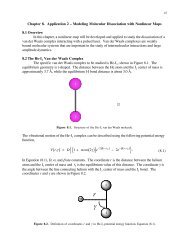
Such a process is illustrated for a system with two geometrical coordinates in Figure 2.
Figure 2. Illustration of the steepest descent method for a system with two geometrical coordinates.
Conjugate Gradient Method
In the Conjugate Gradient method, the first portion of the search takes place opposite the direction of the largest
gradient, just as in the Steepest Descent method. However, to avoid some of the oscillating back and forth that often
plagues the steepest descent method as it moves toward the minimum, the conjugate gradient method mixes in a
little of the previous direction in the next search. This allows the method to move rapidly to the minimum. The
equations for the conjugate gradient method are more complex than those of the other two methods, so they will not
be given here.