Energy Minimization Methods

Chemistry 380.37
May 2013
Dr. Jean M. Standard
May 16, 2013
Energy Minimization Methods
Knowing the stable conformers of a molecule is important because it allows us to understand its properties and
behavior based on its structure. When a molecule is built in a computational chemistry software package, the initial
geometry does not necessarily correspond to one of the stable conformers. Therefore, energy minimization is
usually carried out to determine a stable conformer. This process also is called geometry optimization.
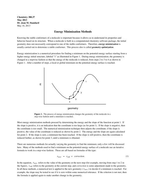
Energy minimization is a numerical procedure for finding a minimum on the potential energy surface starting from a
higher energy initial structure, labeled "1" as illustrated in Figure 1. During energy minimization, the geometry is
changed in a stepwise fashion so that the energy of the molecule is reduced, from steps 2 to 3 to 4 as shown in
Figure 1. After a number of steps, a local or global minimum on the potential energy surface is reached.
E
1
2
4
3
geometry
Figure 1. The process of energy minimization changes the geometry of the molecule in a
step-wise fashion until a minimum is reached.
Most energy minimization methods proceed by determining the energy and the slope of the function at point 1. If
the slope is positive, it is an indication that the coordinate is too large (as for point 1). If the slope is negative, then
the coordinate is too small. The numerical minimization technique then adjusts the coordinate; if the slope is
positive, the value of the coordinate is reduced as shown by point 2. The energy and the slope are again calculated
for point 2. If the slope is zero, a minimum has been reached. If the slope is still positive, then the coordinate is
reduced further, as shown for point 3, until a minimum is obtained.
There are numerous methods for actually varying the geometry to find the minimum; only a few will be discussed
here. Many of the methods used to find a minimum on the potential energy surface of a molecule use an iterative
formula to work in a step-wise fashion. These are all based on formulas of the type:
x new = x old + correction . (1)
In the equation, x new refers to the value of the geometry at the next step (for example, moving from step 1 to 2 in
the figure), x old refers to the geometry at the current step, and correction is some adjustment made to the geometry.
In all these methods, a numerical test is applied to the new geometry ( x new ) to decide if a minimum is reached. For
example, the slope may be tested to see if it is zero within some numerical tolerance. If the criterion is not met, then
the formula is applied again to make another change in the geometry.

2
Newton-Raphson Method
The Newton-Raphson method is the most computationally expensive per step of all the methods utilized to perform
energy minimization. It is based on Taylor series expansion of the potential energy surface at the current geometry.
The equation for updating the geometry is
x new = x old −
( )
( ) . (2)
E ʹ′ x old
E ʹ′ ʹ′ x old
Notice that the correction term depends on both the first derivative (also called the slope or gradient) of the potential
energy surface at the current geometry € and also on the second derivative (otherwise known as the curvature). It is
the necessity of calculating these derivatives at each step that makes the method very expensive per step, especially
for a multidimensional potential energy surface where there are many directions in which to calculate the gradients
and curvatures. However, the Newton-Raphson method usually requires the fewest steps to reach the minimum.
Steepest Descent Method
Rather than requiring the calculation of numerous second derivatives, the steepest descent method relies on an
approximation. In this method, the second derivative is assumed to be a constant. Therefore, the equation to update
the geometry becomes
x new = x old − γ E ʹ′ x old
( ) , (3)
where γ is a constant. In this method, the gradients at each point still must be calculated, but by not requiring second
derivatives to be calculated, the € method is much faster per step than the Newton-Raphson method. However,
because of the approximation, it is not as efficient and so more steps are generally required to find the minimum.
The method is named Steepest Descent because the direction in which the geometry is first minimized is opposite to
the direction in which the gradient is largest (i.e., steepest) at the initial point. Once a minimum in the first direction
is reached, a second minimization is carried out starting from that point and moving in the steepest remaining
direction. This process continues until a minimum has been reached in all directions to within a sufficient tolerance.
Such a process is illustrated for a system with two geometrical coordinates in Figure 2.
Figure 2. Illustration of the steepest descent method for a system with two geometrical coordinates.
Conjugate Gradient Method
In the Conjugate Gradient method, the first portion of the search takes place opposite the direction of the largest
gradient, just as in the Steepest Descent method. However, to avoid some of the oscillating back and forth that often
plagues the steepest descent method as it moves toward the minimum, the conjugate gradient method mixes in a
little of the previous direction in the next search. This allows the method to move rapidly to the minimum. The
equations for the conjugate gradient method are more complex than those of the other two methods, so they will not
be given here.

3
An Example of the Use of Energy Minimization Methods – CPU Times
As an example of these various energy minimization methods, the geometry of lactic acid was optimized using the
Newton-Raphson, Steepest Descent, and Conjugate Gradient methods. Lactic acid is a relatively small organic
molecule shown in Figure 3.
HO
OH
O
Figure 3. lactic acid
The results of the energy minimizations are summarized in Table 1. Each minimization started from the same initial
geometry of lactic acid and used the same force field (MM3).
Table 1. Energy minimization of lactic acid using the MM3 force field
Method No. of Steps Total CPU Time
(sec)
CPU Time/Step
Newton-Raphson 15 14.8 0.99
Conjugate Gradient 72 15.8 0.22
Steepest Descent 500 41.0 0.08
From the table, it is clear that the Newton-Raphson method required the fewest number of steps to reach the
minimum, while the Steepest Descent method required by far the largest number of steps. On the other hand, the
Steepest Descent method requires the smallest amount of CPU time per step, so even though it required 8-30 times
more steps than the other methods, it only required about 2.7-fold more CPU time.
For larger molecules, the expense of the Newton-Raphson method becomes even more pronounced, leading to a
much higher CPU time per step than for the other methods. Even though each step takes the smallest amount of
CPU time of the three methods, the Steepest Descent method requires many more steps to find a minimum, so it is
very inefficient. Therefore, the most commonly used method for energy minimization of large molecules is usually
some form of the Conjugate Gradient method.

4
Energy Minimization Tolerances
An energy minimization usually is carried out on a computer until the gradients (slopes) for all the coordinates are
within some tolerance. For example, the default tolerance may be set so that the absolute value of the gradient must
be less than or equal to 0.1 kcal/mol-Å. This means that in most cases, the computer will not find exactly the
minimum (in the example below, at x=1.000 Å) but something very close.
0.004
Energy (kcal/mol)
0.003
0.002
0.001
0
0.98 0.99 1 1.01 1.02
x (angstroms)
Figure 4. Example potential for bond stretching.
For the example potential in Figure 4, suppose an energy minimization starts out with x=1.06 Å and after a few
steps, it has reached the point x=1.01 Å. At each point in the minimization, the computer checks the gradients
(slopes) to see if the tolerance has been reached. For the point x=1.01 Å in this example, we can estimate the slope
by drawing a tangent line at that point and calculating the slope as Δy/Δx. For x=1.01Å, the slope of the tangent line
comes out to about 0.21 kcal/mol-Å, so the minimization is not complete.
If the minimization then continues for a few more steps and eventually reaches the point x=1.005 Å, an estimate of
the slope of the tangent line at this point yields about –0.10 kcal/mol-Å. Therefore, since the absolute value of the
slope is equal to the tolerance, the minimization would stop. For this example, the computer would find any
geometry within the range of 0.995 – 1.005 Å as being numerically acceptable for the minimized geometry.
If the range of geometries for which the gradient tolerance is satisfied (in this case, 0.005 Å) is too large, the
tolerance can be made smaller in the software package and the minimization can be run again in order to find a
geometry closer to the actual minimum.
In addition to tolerance for the gradient, an energy minimization also usually includes tolerances for the energy.
That is, a check is usually made to ensure that the energy of the minimized structure is the same as the previous step
to within a certain tolerance. For example, a particular minimization might require the energy to be converged to
within 0.01 kJ/mol.

5
Energy Minimization Example: C-C Bond Stretching
The MM3 force field term describing bond stretching is given by
U s = k ( r − r eq ) 2 − w ( r − r eq ) 3 , (4)
where r is the C-C bond distance, r eq is the equilibrium C-C bond distance, k is the stretching force constant, and w
is an anharmonic correction € term to improve the accuracy of the force field. For a C-C single bond, the parameters
are k=317 kcal mol –1 Å –2 , w=30 kcal mol –1 Å –3 , and r eq=1.523 Å.
€
Suppose the initial structure built for a molecule containing a C-C bond has a C-C bond length of 1.900 Å. Tables 2
and 3 show how the energy minimization € progresses for the Newton-Raphson and Steepest Descent methods.
Table 2. Newton-Raphson Energy Minimization
r new = r old −
( )
( )
U ʹ′ r old
U ʹ′ ʹ′ r old
Step
r old U ʹ′
r new
1 € 1.9000 226.23 1.5004
2 1.5004 –14.37 1.5229
3
€
1.5229 € –0.05
€
1.5230
Table 3. Steepest Descent Energy Minimization (with γ = 0.001)
( )
r new = r old − γ U ʹ′ r old
Step
r old U ʹ′
r new
1 € 1.9000 226.23 1.6738
2 1.6738 93.54 1.5802
3
€
1.5802 € 35.99
€
1.5442
4 1.5442 13.43 1.5308
5 1.5308 4.95 1.5259
6 1.5259 1.82 1.5240
7 1.5240 0.67 1.5234
8 1.5234 0.24 1.5231
9 1.5231 0.09 1.52305