NUMERICAL METHODS IN HEAT CONDUCTION So - Kostic

NUMERICAL METHODS
IN HEAT CONDUCTION
CHAPTER
5
So far we have mostly considered relatively simple heat conduction problems
involving simple geometries with simple boundary conditions because
only such simple problems can be solved analytically. But many
problems encountered in practice involve complicated geometries with complex
boundary conditions or variable properties, and cannot be solved analytically.
In such cases, sufficiently accurate approximate solutions can be
obtained by computers using a numerical method.
Analytical solution methods such as those presented in Chapter 2 are based
on solving the governing differential equation together with the boundary conditions.
They result in solution functions for the temperature at every point in
the medium. Numerical methods, on the other hand, are based on replacing the
differential equation by a set of n algebraic equations for the unknown temperatures
at n selected points in the medium, and the simultaneous solution of
these equations results in the temperature values at those discrete points.
There are several ways of obtaining the numerical formulation of a heat
conduction problem, such as the finite difference method, the finite element
method, the boundary element method, and the energy balance (or control
volume) method. Each method has its own advantages and disadvantages, and
each is used in practice. In this chapter, we use primarily the energy balance
approach since it is based on the familiar energy balances on control volumes
instead of heavy mathematical formulations, and thus it gives a better physical
feel for the problem. Besides, it results in the same set of algebraic equations
as the finite difference method. In this chapter, the numerical
formulation and solution of heat conduction problems are demonstrated for
both steady and transient cases in various geometries.
CONTENTS
5–1 Why Numerical Methods 286
5–2 Finite Difference Formulation of
Differential Equations 289
5–3 One-Dimensional
Steady Heat Conduction 292
5–4 Two-Dimensional
Steady Heat Conduction 302
5–5 Transient Heat Conduction 311
Topic of Special Interest:
Controlling the
Numerical Error 329
Summary 333
References and Suggested
Reading 334
Problems 334
OBJECTIVES
When you finish studying this chapter, you should be able to:
■ Understand the limitations of analytical solutions of conduction problems, and the need
for computation-intensive numerical methods,
■ Express derivates as differences, and obtain finite difference formulations,
■ Solve steady one- or two-dimensional conduction problems numerically using the finite
difference method, and
■ Solve transient one- or two-dimensional conduction problems using the finite difference
method.
285

286
NUMERICAL METHODS
( )
1 d
r 2 dT
+ ——
e·
— — —dr = 0
r 2 dr k
Sphere
dT(0)
——–
dr
= 0
Solution:
T(r) = T (r2 o – r 2 1 + ——
e
)
6k·
0
T(r o ) = T 1
· dT 4 π r 3 e·
Q(r) = –kA —dr = ———
3
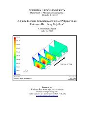
FIGURE 5–1
The analytical solution of a problem
requires solving the governing
differential equation and applying
the boundary conditions.
r o
■
5–1 WHY NUMERICAL METHODS
The ready availability of high-speed computers and easy-to-use powerful software
packages has had a major impact on engineering education and practice
in recent years. Engineers in the past had to rely on analytical skills to solve
significant engineering problems, and thus they had to undergo a rigorous
training in mathematics. Today’s engineers, on the other hand, have access to
a tremendous amount of computation power under their fingertips, and they
mostly need to understand the physical nature of the problem and interpret the
results. But they also need to understand how calculations are performed by
the computers to develop an awareness of the processes involved and the limitations,
while avoiding any possible pitfalls.
In Chapter 2, we solved various heat conduction problems in various geometries
in a systematic but highly mathematical manner by (1) deriving the
governing differential equation by performing an energy balance on a differential
volume element, (2) expressing the boundary conditions in the proper
mathematical form, and (3) solving the differential equation and applying the
boundary conditions to determine the integration constants. This resulted in a
solution function for the temperature distribution in the medium, and the solution
obtained in this manner is called the analytical solution of the problem.
For example, the mathematical formulation of one-dimensional steady heat
conduction in a sphere of radius r o whose outer surface is maintained at a uniform
temperature of T 1 with uniform heat generation at a rate of e· was expressed
as (Fig. 5–1)
whose (analytical) solution is
1
e # 0
r dr d r 2 dT
dr
2 k
dT(0)
0 and T(r o ) T 1 (5–1)
dr
e #
T(r) T 1 r 2 ) (5–2)
6k (r o
2
This is certainly a very desirable form of solution since the temperature at
any point within the sphere can be determined simply by substituting the
r-coordinate of the point into the analytical solution function above. The analytical
solution of a problem is also referred to as the exact solution since it
satisfies the differential equation and the boundary conditions. This can be
verified by substituting the solution function into the differential equation and
the boundary conditions. Further, the rate of heat transfer at any location
within the sphere or its surface can be determined by taking the derivative of
the solution function T(r) and substituting it into Fourier’s law as
dT
Q· (r) kA k(4pr 2 4pr 3 e #
) a e# r
(5–3)
dr
3k b 3
The analysis above did not require any mathematical sophistication beyond
the level of simple integration, and you are probably wondering why anyone

would ask for something else. After all, the solutions obtained are exact and
easy to use. Besides, they are instructive since they show clearly the functional
dependence of temperature and heat transfer on the independent variable r.
Well, there are several reasons for searching for alternative solution methods.
287
CHAPTER 5
1 Limitations
Analytical solution methods are limited to highly simplified problems in simple
geometries (Fig. 5–2). The geometry must be such that its entire surface
can be described mathematically in a coordinate system by setting the variables
equal to constants. That is, it must fit into a coordinate system perfectly
with nothing sticking out or in. In the case of one-dimensional heat conduction
in a solid sphere of radius r o , for example, the entire outer surface can be
described by r r o . Likewise, the surfaces of a finite solid cylinder of radius
r o and height H can be described by r r o for the side surface and z 0 and
z H for the bottom and top surfaces, respectively. Even minor complications
in geometry can make an analytical solution impossible. For example, a spherical
object with an extrusion like a handle at some location is impossible to
handle analytically since the boundary conditions in this case cannot be expressed
in any familiar coordinate system.
Even in simple geometries, heat transfer problems cannot be solved analytically
if the thermal conditions are not sufficiently simple. For example, the
consideration of the variation of thermal conductivity with temperature, the
variation of the heat transfer coefficient over the surface, or the radiation heat
transfer on the surfaces can make it impossible to obtain an analytical solution.
Therefore, analytical solutions are limited to problems that are simple or
can be simplified with reasonable approximations.
2 Better Modeling
We mentioned earlier that analytical solutions are exact solutions since they
do not involve any approximations. But this statement needs some clarification.
Distinction should be made between an actual real-world problem and
the mathematical model that is an idealized representation of it. The solutions
we get are the solutions of mathematical models, and the degree of applicability
of these solutions to the actual physical problems depends on the accuracy
of the model. An “approximate” solution of a realistic model of a
physical problem is usually more accurate than the “exact” solution of a crude
mathematical model (Fig. 5–3).
When attempting to get an analytical solution to a physical problem, there
is always the tendency to oversimplify the problem to make the mathematical
model sufficiently simple to warrant an analytical solution. Therefore, it is
common practice to ignore any effects that cause mathematical complications
such as nonlinearities in the differential equation or the boundary conditions.
So it comes as no surprise that nonlinearities such as temperature dependence
of thermal conductivity and the radiation boundary conditions are seldom considered
in analytical solutions. A mathematical model intended for a numerical
solution is likely to represent the actual problem better. Therefore, the
numerical solution of engineering problems has now become the norm rather
than the exception even when analytical solutions are available.
T , h
No
radiation
T , h
Simplified
model
k = constant
Long
cylinder
h = constant
T = constant
h, T
No
radiation
h, T
FIGURE 5–2
Analytical solution methods are
limited to simplified problems
in simple geometries.
A sphere
Exact (analytical)
solution of model,
but crude solution
of actual problem
An
oval-shaped
body
Realistic
model
Approximate (numerical)
solution of model,
but accurate solution
of actual problem
FIGURE 5–3
The approximate numerical solution
of a real-world problem may be more
accurate than the exact (analytical)
solution of an oversimplified
model of that problem.

288
NUMERICAL METHODS
T(r, z)
z
L
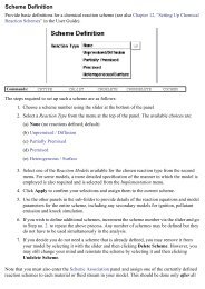
3 Flexibility
Engineering problems often require extensive parametric studies to understand
the influence of some variables on the solution in order to choose the
right set of variables and to answer some “what-if ” questions. This is an iterative
process that is extremely tedious and time-consuming if done by hand.
Computers and numerical methods are ideally suited for such calculations,
and a wide range of related problems can be solved by minor modifications in
the code or input variables. Today it is almost unthinkable to perform any significant
optimization studies in engineering without the power and flexibility
of computers and numerical methods.
T
r
0
T 0
Analytical solution:
T(r, z) – T
= ∑
J
————– 0 ( λ n r) sinh λ
———— n (L – z)
T 0 – T
λ
n=1 n J 1 ( λn r o ) –—————
sinh ( λ n L)
r o
where λ n ’s are roots of J 0 ( λ n r o ) = 0
FIGURE 5–4
Some analytical solutions are very
complex and difficult to use.
FIGURE 5–5
The ready availability of high-powered
computers with sophisticated software
packages has made numerical solution
the norm rather than the exception.
4 Complications
Some problems can be solved analytically, but the solution procedure is so
complex and the resulting solution expressions so complicated that it is not
worth all that effort. With the exception of steady one-dimensional or transient
lumped system problems, all heat conduction problems result in partial
differential equations. Solving such equations usually requires mathematical
sophistication beyond that acquired at the undergraduate level, such as orthogonality,
eigenvalues, Fourier and Laplace transforms, Bessel and Legendre
functions, and infinite series. In such cases, the evaluation of the solution,
which often involves double or triple summations of infinite series at a specified
point, is a challenge in itself (Fig. 5–4). Therefore, even when the solutions
are available in some handbooks, they are intimidating enough to scare
prospective users away.
5 Human Nature
As human beings, we like to sit back and make wishes, and we like our wishes
to come true without much effort. The invention of TV remote controls made
us feel like kings in our homes since the commands we give in our comfortable
chairs by pressing buttons are immediately carried out by the obedient
TV sets. After all, what good is cable TV without a remote control. We certainly
would love to continue being the king in our little cubicle in the engineering
office by solving problems at the press of a button on a computer
(until they invent a remote control for the computers, of course). Well, this
might have been a fantasy yesterday, but it is a reality today. Practically all
engineering offices today are equipped with high-powered computers with
sophisticated software packages, with impressive presentation-style colorful
output in graphical and tabular form (Fig. 5–5). Besides, the results are as
accurate as the analytical results for all practical purposes. The computers
have certainly changed the way engineering is practiced.
The discussions above should not lead you to believe that analytical solutions
are unnecessary and that they should be discarded from the engineering
curriculum. On the contrary, insight to the physical phenomena and engineering
wisdom is gained primarily through analysis. The “feel” that engineers
develop during the analysis of simple but fundamental problems serves as
an invaluable tool when interpreting a huge pile of results obtained from a
computer when solving a complex problem. A simple analysis by hand for
a limiting case can be used to check if the results are in the proper range. Also,

nothing can take the place of getting “ball park” results on a piece of paper
during preliminary discussions. The calculators made the basic arithmetic
operations by hand a thing of the past, but they did not eliminate the need for
instructing grade school children how to add or multiply.
In this chapter, you will learn how to formulate and solve heat transfer
problems numerically using one or more approaches. In your professional life,
you will probably solve the heat transfer problems you come across using a
professional software package, and you are highly unlikely to write your own
programs to solve such problems. (Besides, people will be highly skeptical
of the results obtained using your own program instead of using a wellestablished
commercial software package that has stood the test of time.) The
insight you gain in this chapter by formulating and solving some heat transfer
problems will help you better understand the available software packages and
be an informed and responsible user.
289
CHAPTER 5
5–2
■
FINITE DIFFERENCE FORMULATION
OF DIFFERENTIAL EQUATIONS
The numerical methods for solving differential equations are based on replacing
the differential equations by algebraic equations. In the case of the popular
finite difference method, this is done by replacing the derivatives by
differences. Below we demonstrate this with both first- and second-order
derivatives. But first we give a motivational example.
Consider a man who deposits his money in the amount of A 0 $100 in a
savings account at an annual interest rate of 18 percent, and let us try to determine
the amount of money he will have after one year if interest is compounded
continuously (or instantaneously). In the case of simple interest, the
money will earn $18 interest, and the man will have 100 100 0.18
$118.00 in his account after one year. But in the case of compounding, the
interest earned during a compounding period will also earn interest for the
remaining part of the year, and the year-end balance will be greater than $118.
For example, if the money is compounded twice a year, the balance will be
100 100 (0.18/2) $109 after six months, and 109 109 (0.18/2)
$118.81 at the end of the year. We could also determine the balance A directly
from
A A 0 (1 i) n ($100)(1 0.09) 2 $118.81 (5–4)
where i is the interest rate for the compounding period and n is the number of
periods. Using the same formula, the year-end balance is determined for
monthly, daily, hourly, minutely, and even secondly compounding, and the
results are given in Table 5–1.
Note that in the case of daily compounding, the year-end balance will be
$119.72, which is $1.72 more than the simple interest case. (So it is no wonder
that the credit card companies usually charge interest compounded daily when
determining the balance.) Also note that compounding at smaller time intervals,
even at the end of each second, does not change the result, and we suspect
that instantaneous compounding using “differential” time intervals dt will
give the same result. This suspicion is confirmed by obtaining the differential
TABLE 5–1
Year-end balance of a $100 account
earning interest at an annual rate
of 18 percent for various
compounding periods
Number
Compounding of Year-End
Period Periods, n Balance
1 year 1 $118.00
6 months 2 118.81
1 month 12 119.56
1 week 52 119.68
1 day 365 119.72
1 hour 8760 119.72
1 minute 525,600 119.72
1 second 31,536,000 119.72
Instantaneous 119.72

290
NUMERICAL METHODS
equation dA/dt iA for the balance A, whose solution is A A 0 exp(it). Substitution
yields
A ($100)exp(0.18 1) $119.72
f(x)
f(x + ∆x)
f(x)
∆x
∆f
which is identical to the result for daily compounding. Therefore, replacing a
differential time interval dt by a finite time interval of t 1 day gave the
same result when rounded to the second decimal place for cents, which leads
us into believing that reasonably accurate results can be obtained by replacing
differential quantities by sufficiently small differences.
Next, we develop the finite difference formulation of heat conduction problems
by replacing the derivatives in the differential equations by differences.
In the following section we do it using the energy balance method, which does
not require any knowledge of differential equations.
Derivatives are the building blocks of differential equations, and thus we
first give a brief review of derivatives. Consider a function f that depends on x,
as shown in Figure 5–6. The first derivative of f(x) at a point is equivalent to
the slope of a line tangent to the curve at that point and is defined as
Tangent line
x x + ∆x x
FIGURE 5–6
The derivative of a function at a point
represents the slope of the function
at that point.
T m + 1
T m
T m – 1
Plane wall
T(x)
L
0
0 1 2 … m–1 m m+1…
M
M–1
m–
1
–
2 m+ 1 – 2
FIGURE 5–7
Schematic of the nodes and the nodal
temperatures used in the development
of the finite difference formulation
of heat transfer in a plane wall.
x
df(x)
dx
f f(x x) f(x)
lim lim
(5–5)
x → 0 x x → 0 x
which is the ratio of the increment f of the function to the increment x of the
independent variable as x → 0. If we don’t take the indicated limit, we will
have the following approximate relation for the derivative:
df(x)
dx
f(x x) f(x)
x
(5–6)
This approximate expression of the derivative in terms of differences is the
finite difference form of the first derivative. The equation above can also be
obtained by writing the Taylor series expansion of the function f about the
point x,
df(x) 1 d 2 f(x)
f(x x) f(x) x x 2 · · · (5–7)
dx 2 dx 2
and neglecting all the terms in the expansion except the first two. The first
term neglected is proportional to x 2 , and thus the error involved in each step
of this approximation is also proportional to x 2 . However, the commutative
error involved after M steps in the direction of length L is proportional to x
since Mx 2 (L/x)x 2 Lx. Therefore, the smaller the x, the smaller
the error, and thus the more accurate the approximation.
Now consider steady one-dimensional heat conduction in a plane wall of
thickness L with heat generation. The wall is subdivided into M sections of
equal thickness x L/M in the x-direction, separated by planes passing
through M 1 points 0, 1, 2, . . . , m 1, m, m 1, . . . , M called nodes or
nodal points, as shown in Figure 5–7. The x-coordinate of any point m is simply
x m mx, and the temperature at that point is simply T(x m ) T m .
The heat conduction equation involves the second derivatives of temperature
with respect to the space variables, such as d 2 T/dx 2 , and the finite difference
formulation is based on replacing the second derivatives by appropriate

differences. But we need to start the process with first derivatives. Using
1
Eq. 5–6, the first derivative of temperature dT/dx at the midpoints m and
2
m of the sections surrounding the node m can be expressed as
1
2
291
CHAPTER 5
Noting that the second derivative is simply the derivative of the first derivative,
the second derivative of temperature at node m can be expressed as
d 2 T
dx 2 m
dT T m T m1
dT T m1 T m
and (5–8)
dx 1
x
dx 1
m m x
2
2
dT
T m1 T m
T m T m1
dx 1
dT
m dx 1 m
2
2 x x
x
x
T m1 2T m T m1
x 2
(5–9)
which is the finite difference representation of the second derivative at a general
internal node m. Note that the second derivative of temperature at a node
m is expressed in terms of the temperatures at node m and its two neighboring
nodes. Then the differential equation
T e # m1 2T m T m1 m
0,
x 2 k
m 1, 2, 3, . . . , M 1 (5–11)
d 2 T e #
0
dx 2 k
(5–10)
which is the governing equation for steady one-dimensional heat transfer in a
plane wall with heat generation and constant thermal conductivity, can be expressed
in the finite difference form as (Fig. 5–8)
where e·m is the rate of heat generation per unit volume at node m. If the surface
temperatures T 0 and T M are specified, the application of this equation
to each of the M 1 interior nodes results in M 1 equations for the determination
of M 1 unknown temperatures at the interior nodes. Solving
these equations simultaneously gives the temperature values at the nodes. If
the temperatures at the outer surfaces are not known, then we need to obtain
two more equations in a similar manner using the specified boundary conditions.
Then the unknown temperatures at M 1 nodes are determined by
solving the resulting system of M 1 equations in M 1 unknowns simultaneously.
Note that the boundary conditions have no effect on the finite difference formulation
of interior nodes of the medium. This is not surprising since the control
volume used in the development of the formulation does not involve any
part of the boundary. You may recall that the boundary conditions had no
effect on the differential equation of heat conduction in the medium either.
The finite difference formulation above can easily be extended to two- or
three-dimensional heat transfer problems by replacing each second derivative
by a difference equation in that direction. For example, the finite difference
formulation for steady two-dimensional heat conduction in a region with
Plane wall
Differential equation:
d 2 T e·
—– + —— = 0
dx 2 k
Valid at every point
Finite difference equation:
T m – 1 – 2T m + T e·
—–——————— m + 1
+ — m
= 0
∆x 2 k
Valid at discrete points
∆x
FIGURE 5–8
The differential equation is valid at
every point of a medium, whereas the
finite difference equation is valid at
discrete points (the nodes) only.

n + 1
y
n
n – 1
x
292
NUMERICAL METHODS
∆y m – 1, n
∆y
m, n + 1
m, n m + 1, n
m, n – 1
∆x
∆x
m – 1 m m + 1
FIGURE 5–9
Finite difference mesh for twodimensional
conduction in
rectangular coordinates.
0
0
Plane wall
·
Q cond, left
Volume
element
of node m
A general
interior node
L
1 2 m – 1 m m + 1 M x
∆x
e·
m
∆x
∆x
·
Q cond, right
FIGURE 5–10
The nodal points and volume
elements for the finite difference
formulation of one-dimensional
conduction in a plane wall.
heat generation and constant thermal conductivity can be expressed in rectangular
coordinates as (Fig. 5–9)
T e # m1, n 2T m, n T m1, n T m, n1 2T m, n T m, n1 m, n
0 (5–12)
x 2
y 2
k
for m 1, 2, 3, . . . , M 1 and n 1, 2, 3, . . . , N 1 at any interior node
(m, n). Note that a rectangular region that is divided into M equal subregions
in the x-direction and N equal subregions in the y-direction has a total of
(M 1)(N 1) nodes, and Eq. 5–12 can be used to obtain the finite difference
equations at (M 1)(N 1) of these nodes (i.e., all nodes except those
at the boundaries).
The finite difference formulation is given above to demonstrate how difference
equations are obtained from differential equations. However, we use the
energy balance approach in the following sections to obtain the numerical formulation
because it is more intuitive and can handle boundary conditions
more easily. Besides, the energy balance approach does not require having the
differential equation before the analysis.
5–3
■
ONE-DIMENSIONAL
STEADY HEAT CONDUCTION
In this section we develop the finite difference formulation of heat conduction
in a plane wall using the energy balance approach and discuss how to solve
the resulting equations. The energy balance method is based on subdividing
the medium into a sufficient number of volume elements and then applying an
energy balance on each element. This is done by first selecting the nodal
points (or nodes) at which the temperatures are to be determined and then
forming elements (or control volumes) over the nodes by drawing lines
through the midpoints between the nodes. This way, the interior nodes remain
at the middle of the elements, and the properties at the node such as the
temperature and the rate of heat generation represent the average properties of
the element. Sometimes it is convenient to think of temperature as varying
linearly between the nodes, especially when expressing heat conduction between
the elements using Fourier’s law.
To demonstrate the approach, again consider steady one-dimensional heat
transfer in a plane wall of thickness L with heat generation e·(x) and constant
conductivity k. The wall is now subdivided into M equal regions of thickness
x L/M in the x-direction, and the divisions between the regions are
selected as the nodes. Therefore, we have M 1 nodes labeled 0, 1, 2, . . . ,
m 1, m, m 1, . . . , M, as shown in Figure 5–10. The x-coordinate of any
node m is simply x m mx, and the temperature at that point is T(x m ) T m .
Elements are formed by drawing vertical lines through the midpoints between
the nodes. Note that all interior elements represented by interior nodes are
full-size elements (they have a thickness of x), whereas the two elements at
the boundaries are half-sized.
To obtain a general difference equation for the interior nodes, consider the
element represented by node m and the two neighboring nodes m 1 and
m 1. Assuming the heat conduction to be into the element on all surfaces,
an energy balance on the element can be expressed as

Rate of heat
conduction
at the left
surface
Rate of heat Rate of heat
conduction generation
at the right inside the
surface element
Rate of change
of the energy
content of
the element
293
CHAPTER 5
or
E element
Q· cond, left Q· cond, right E·gen, element 0 (5–13)
t
since the energy content of a medium (or any part of it) does not change under
steady conditions and thus E element 0. The rate of heat generation within
the element can be expressed as
E·gen, element e·mV element e·m Ax (5–14)
where e·m is the rate of heat generation per unit volume in W/m 3 evaluated at
node m and treated as a constant for the entire element, and A is heat transfer
area, which is simply the inner (or outer) surface area of the wall.
Recall that when temperature varies linearly, the steady rate of heat conduction
across a plane wall of thickness L can be expressed as
T
Q· cond kA (5–15)
L
where T is the temperature change across the wall and the direction of heat
transfer is from the high temperature side to the low temperature. In the case
of a plane wall with heat generation, the variation of temperature is not linear
and thus the relation above is not applicable. However, the variation of temperature
between the nodes can be approximated as being linear in the determination
of heat conduction across a thin layer of thickness x between two
nodes (Fig. 5–11). Obviously the smaller the distance x between two nodes,
the more accurate is this approximation. (In fact, such approximations are the
reason for classifying the numerical methods as approximate solution methods.
In the limiting case of x approaching zero, the formulation becomes exact
and we obtain a differential equation.) Noting that the direction of heat
transfer on both surfaces of the element is assumed to be toward the node m,
the rate of heat conduction at the left and right surfaces can be expressed as
Linear
m – 1
∆x
k
m
Volume
element
T m
T m + 1
∆x
m + 1
Linear
T m – 1
FIGURE 5–11
T m1 T m
T m1 T m
Q· cond, left kA and Q· cond, right kA (5–16)
x
x
Substituting Eqs. 5–14 and 5–16 into Eq. 5–13 gives
kA————–
T m – 1 – T m
∆x
A
kA————–
T m + 1 – T m
∆x
A
T m1 T m T m1 T m
kA kA e·m Ax 0 (5–17)
x
x
which simplifies to
In finite difference formulation, the
temperature is assumed to vary
linearly between the nodes.
T e # m1 2T m T m1 m
0, m 1, 2, 3, . . . , M 1 (5–18)
x 2 k

or
kA———
T 1 – T 2
∆x
294
NUMERICAL METHODS
T
kA 1 – T
——— 2
∆x
e·
2 A∆x
1 2
3
Volume
element
of node 2
kA———
T 2 – T 3
∆x
(a) Assuming heat transfer to be out of the
volume element at the right surface.
or
kA———
T 1 – T 2
∆x
– kA———
T 2 – T 3
+ e·
∆x 2 A∆x = 0
T 1 – 2T 2 + T 3 + e·
2 A∆x 2 / k = 0
T
kA 1 – T
——— 2
∆x
e·
2 A∆x
1 2
3
Volume
element
of node 2
kA———
T 3 – T 2
∆x
+ kA———
T 3 – T 2
+ e·
∆x 2 A∆x = 0
T 1 – 2T 2 + T 3 + e·
2 A∆x 2 / k = 0
(b) Assuming heat transfer to be into the
volume element at all surfaces.
FIGURE 5–12
The assumed direction of heat transfer
at surfaces of a volume element has
no effect on the finite difference
formulation.
which is identical to the difference equation (Eq. 5–11) obtained earlier.
Again, this equation is applicable to each of the M 1 interior nodes, and its
application gives M 1 equations for the determination of temperatures at
M 1 nodes. The two additional equations needed to solve for the M 1 unknown
nodal temperatures are obtained by applying the energy balance on the
two elements at the boundaries (unless, of course, the boundary temperatures
are specified).
You are probably thinking that if heat is conducted into the element from
both sides, as assumed in the formulation, the temperature of the medium will
have to rise and thus heat conduction cannot be steady. Perhaps a more realistic
approach would be to assume the heat conduction to be into the element on
the left side and out of the element on the right side. If you repeat the formulation
using this assumption, you will again obtain the same result since the
heat conduction term on the right side in this case involves T m T m 1 instead
of T m 1 T m , which is subtracted instead of being added. Therefore, the assumed
direction of heat conduction at the surfaces of the volume elements has
no effect on the formulation, as shown in Figure 5–12. (Besides, the actual direction
of heat transfer is usually not known.) However, it is convenient to assume
heat conduction to be into the element at all surfaces and not worry
about the sign of the conduction terms. Then all temperature differences in
conduction relations are expressed as the temperature of the neighboring node
minus the temperature of the node under consideration, and all conduction
terms are added.
Boundary Conditions
Above we have developed a general relation for obtaining the finite difference
equation for each interior node of a plane wall. This relation is not applicable
to the nodes on the boundaries, however, since it requires the presence of
nodes on both sides of the node under consideration, and a boundary node
does not have a neighboring node on at least one side. Therefore, we need to
obtain the finite difference equations of boundary nodes separately. This is
best done by applying an energy balance on the volume elements of boundary
nodes.
Boundary conditions most commonly encountered in practice are the specified
temperature, specified heat flux, convection, and radiation boundary conditions,
and here we develop the finite difference formulations for them for the
case of steady one-dimensional heat conduction in a plane wall of thickness L
as an example. The node number at the left surface at x 0 is 0, and at the
right surface at x L it is M. Note that the width of the volume element for either
boundary node is x/2.
The specified temperature boundary condition is the simplest boundary
condition to deal with. For one-dimensional heat transfer through a plane wall
of thickness L, the specified temperature boundary conditions on both the left
and right surfaces can be expressed as (Fig. 5–13)
T(0) T 0 Specified value
T(L) T M Specified value (5–19)
where T 0 and T M are the specified temperatures at surfaces at x 0 and x L,
respectively. Therefore, the specified temperature boundary conditions are

295
CHAPTER 5
incorporated by simply assigning the given surface temperatures to the boundary
nodes. We do not need to write an energy balance in this case unless we
decide to determine the rate of heat transfer into or out of the medium after the
temperatures at the interior nodes are determined.
When other boundary conditions such as the specified heat flux, convection,
radiation, or combined convection and radiation conditions are specified at a
boundary, the finite difference equation for the node at that boundary is obtained
by writing an energy balance on the volume element at that boundary.
The energy balance is again expressed as
35°C
0
0
1
Plane wall
2
…
82°C
L
M
a
All sides
Q· E·gen, element 0 (5–20)
for heat transfer under steady conditions. Again we assume all heat transfer to
be into the volume element from all surfaces for convenience in formulation,
except for specified heat flux since its direction is already specified. Specified
heat flux is taken to be a positive quantity if into the medium and a negative
quantity if out of the medium. Then the finite difference formulation at the
node m 0 (at the left boundary where x 0) of a plane wall of thickness
L during steady one-dimensional heat conduction can be expressed as
(Fig. 5–14)
T 1 T 0
Q· left surface kA e·0(Ax/2) 0 (5–21)
x
where Ax/2 is the volume of the volume element (note that the boundary element
has half thickness), e·0 is the rate of heat generation per unit volume (in
W/m 3 ) at x 0, and A is the heat transfer area, which is constant for a plane
wall. Note that we have x in the denominator of the second term instead of
x/2. This is because the ratio in that term involves the temperature difference
between nodes 0 and 1, and thus we must use the distance between those two
nodes, which is x.
The finite difference form of various boundary conditions can be obtained
from Eq. 5–21 by replacing Q· left surface by a suitable expression. Next this is
done for various boundary conditions at the left boundary.
1. Specified Heat Flux Boundary Condition
·
Q left surface
T 0 = 35°C
T M = 82°C
FIGURE 5–13
Finite difference formulation of
specified temperature boundary
conditions on both surfaces
of a plane wall.
—–
∆x
2
e·
0
0
0
∆x
Volume element
of node 0
1
kA———
T 1 – T 0
∆x
∆x
L
2 … x
·
Q left surface + kA———
T 1 – T 0 —–
∆x
+ e· ∆x 0 A = 0 2
FIGURE 5–14
Schematic for the finite difference
formulation of the left boundary
node of a plane wall.
T 1 T 0
q·0A kA e·0(Ax/2) 0 (5–22)
x
Special case: Insulated Boundary (q·0 0)
T 1 T 0
kA e·0(Ax/2) 0 (5–23)
x
2. Convection Boundary Condition
T 1 T 0
hA(T T 0 ) kA e·0(Ax/2) 0 (5–24)
x

296
NUMERICAL METHODS
T surr
ε
A(T 4 surr – T 4 0 )
—–
∆x
2
e·
0
3. Radiation Boundary Condition
T 1 T 0
esA( Tsurr 4 T 0
4 ) kA e·0(Ax/2) 0 (5–25)
x
4. Combined Convection and Radiation Boundary Condition
(Fig. 5–15)
εσ
kA———
T 1 – T 0
∆x
hA(T – T 0 )
L
0
0 1 2 … x
A ∆x ∆x
hA(T – T 0 ) + εσ A(T 4 surr – T 4 0 )
T 1 – T
——— 0 ∆x
+ kA + e· —–
∆x 0 A = 0 2
FIGURE 5–15
Schematic for the finite difference
formulation of combined convection
and radiation on the left boundary
of a plane wall.
A
Medium A
k A
k A A ————–
T m – 1 – T m
∆x
e·
· A, m
k B A ————–
T m + 1 – T m
∆x
m – 1 m m + 1 x
∆x ∆x
∆x
—–
∆x
—– 2
2
e B, m
Interface
Medium B
k B
T m – 1 – T ————– m T
k A A
m + 1 – T
+ k m
∆x B A ————–
∆x
∆x
—–
∆x
+ e·
—– + e· A, m A B, m A = 0
2 2
FIGURE 5–16
Schematic for the finite difference
formulation of the interface boundary
condition for two mediums A and B
that are in perfect thermal contact.
A
or
T 1 T 0
hA(T T 0 ) esA( Tsurr 4 T 0
4 ) kA e·0(Ax/2) 0 (5–26)
x
T 1 T 0
h combined A(T T 0 ) kA e·0(Ax/2) 0 (5–27)
x
5. Combined Convection, Radiation, and Heat Flux Boundary
Condition
T 1 T 0
q·0A hA(T T 0 ) esA( Tsurr 4 T0
4 ) kA e·0(Ax/2) 0 (5–28)
x
6. Interface Boundary Condition Two different solid media A and B are
assumed to be in perfect contact, and thus at the same temperature at the
interface at node m (Fig. 5–16). Subscripts A and B indicate properties
of media A and B, respectively.
T m1 T m T m1 T m
k A A k B A e·A, m(Ax/2) e·B, m(Ax/2) 0 (5–29)
x
x
In these relations, q·0 is the specified heat flux in W/m 2 , h is the convection
coefficient, h combined is the combined convection and radiation coefficient, T is
the temperature of the surrounding medium, T surr is the temperature of the
surrounding surfaces, e is the emissivity of the surface, and s is the Stefan–
Boltzman constant. The relations above can also be used for node M on the
right boundary by replacing the subscript “0” by “M” and the subscript “1” by
“M 1”.
Note that thermodynamic temperatures must be used in radiation heat transfer
calculations, and all temperatures should be expressed in K or R when a
boundary condition involves radiation to avoid mistakes. We usually try to
avoid the radiation boundary condition even in numerical solutions since it
causes the finite difference equations to be nonlinear, which are more difficult
to solve.
Treating Insulated Boundary Nodes as Interior Nodes:
The Mirror Image Concept
One way of obtaining the finite difference formulation of a node on an insulated
boundary is to treat insulation as “zero” heat flux and to write an energy
balance, as done in Eq. 5–23. Another and more practical way is to treat the
node on an insulated boundary as an interior node. Conceptually this is done

T e # e # m1 2T m T m1 m T 1 2T 0 T 1
Mirror
0 →
0
0 (5–30)
x 2 k
x 2 k
CHAPTER 5
by replacing the insulation on the boundary by a mirror and considering the
reflection of the medium as its extension (Fig. 5–17). This way the node next
to the boundary node appears on both sides of the boundary node because of
Insulation
symmetry, converting it into an interior node. Then using the general formula
(Eq. 5–18) for an interior node, which involves the sum of the temperatures of
the adjoining nodes minus twice the node temperature, the finite difference
0 1
formulation of a node m 0 on an insulated boundary of a plane wall can be
expressed as
Mirror
which is equivalent to Eq. 5–23 obtained by the energy balance approach.
The mirror image approach can also be used for problems that possess thermal
symmetry by replacing the plane of symmetry by a mirror. Alternately, we
can replace the plane of symmetry by insulation and consider only half of the
medium in the solution. The solution in the other half of the medium is simply
the mirror image of the solution obtained.
297
x 2 1 0 1
Insulated
boundary
node
2
Equivalent
interior
node
FIGURE 5–17
A node on an insulated boundary
can be treated as an interior node by
replacing the insulation by a mirror.
2
x
x
EXAMPLE 5–1
Steady Heat Conduction in a Large
Uranium Plate
Consider a large uranium plate of thickness L 4 cm and thermal conductivity
k 28 W/m · °C in which heat is generated uniformly at a constant rate of
e· 5 10 6 W/m 3 . One side of the plate is maintained at 0°C by iced water
while the other side is subjected to convection to an environment at T 30°C
with a heat transfer coefficient of h 45 W/m 2 · °C, as shown in Figure 5–18.
Considering a total of three equally spaced nodes in the medium, two at the
boundaries and one at the middle, estimate the exposed surface temperature
of the plate under steady conditions using the finite difference approach.
SOLUTION A uranium plate is subjected to specified temperature on one side
and convection on the other. The unknown surface temperature of the plate is
to be determined numerically using three equally spaced nodes.
Assumptions 1 Heat transfer through the wall is steady since there is no indication
of any change with time. 2 Heat transfer is one-dimensional since
the plate is large relative to its thickness. 3 Thermal conductivity is constant.
4 Radiation heat transfer is negligible.
Properties The thermal conductivity is given to be k 28 W/m · °C.
Analysis The number of nodes is specified to be M 3, and they are chosen
to be at the two surfaces of the plate and the midpoint, as shown in the figure.
Then the nodal spacing x becomes
L 0.04 m
x 0.02 m
M 1 3 1
We number the nodes 0, 1, and 2. The temperature at node 0 is given to be
T 0 0°C, and the temperatures at nodes 1 and 2 are to be determined. This
problem involves only two unknown nodal temperatures, and thus we need to
have only two equations to determine them uniquely. These equations are obtained
by applying the finite difference method to nodes 1 and 2.
0°C
0
0
Uranium
plate
k = 28 W/m·°C
e · = 5 × 10 6 W/m 3
h
T
L
1 2 x
FIGURE 5–18
Schematic for Example 5–1.

298
NUMERICAL METHODS
Node 1 is an interior node, and the finite difference formulation at that node
is obtained directly from Eq. 5–18 by setting m 1:
T 0 2T 1 T 2
x 2
e # e # e # 1x 2
1
0 2T 1 T 2 1
0 → 0 → 2T 1 T 2
k
x 2 k
k
(1)
Node 2 is a boundary node subjected to convection, and the finite difference
formulation at that node is obtained by writing an energy balance on the volume
element of thickness x/2 at that boundary by assuming heat transfer to
be into the medium at all sides:
T 1 T 2
hA(T T 2 ) kA e·2(Ax/2) 0
x
Canceling the heat transfer area A and rearranging give
hx e # 2x
T 1 2
1 hx T 2 T (2)
k k 2k
Equations (1) and (2) form a system of two equations in two unknowns T 1 and
T 2 . Substituting the given quantities and simplifying gives
2T 1 T 2 71.43
T 1 1.032T 2 36.68
(in °C)
(in °C)
This is a system of two algebraic equations in two unknowns and can be solved
easily by the elimination method. Solving the first equation for T 1 and substituting
into the second equation result in an equation in T 2 whose solution is
T 2 136.1°C
Plate
h
T
0 1 2 x
2 cm 2 cm
Finite difference solution:
Exact solution:
T 2 = 136.1°C
T 2 = 136.0°C
FIGURE 5–19
Despite being approximate in nature,
highly accurate results can be
obtained by numerical methods.
This is the temperature of the surface exposed to convection, which is the
desired result. Substitution of this result into the first equation gives T 1
103.8°C, which is the temperature at the middle of the plate.
Discussion The purpose of this example is to demonstrate the use of the finite
difference method with minimal calculations, and the accuracy of the result
was not a major concern. But you might still be wondering how accurate the result
obtained above is. After all, we used a mesh of only three nodes for the
entire plate, which seems to be rather crude. This problem can be solved analytically
as described in Chapter 2, and the analytical (exact) solution can be
shown to be
T(x)
0.5e # hL 2 /k e # L T h
hL k
Substituting the given quantities, the temperature of the exposed surface of
the plate at x L 0.04 m is determined to be 136.0°C, which is almost
identical to the result obtained here with the approximate finite difference
method (Fig. 5–19). Therefore, highly accurate results can be obtained with
numerical methods by using a limited number of nodes.
x
e # x 2
2k

299
CHAPTER 5
EXAMPLE 5–2
Heat Transfer from Triangular Fins
Consider an aluminum alloy fin (k 180 W/m · °C) of triangular cross section
with length L 5 cm, base thickness b 1 cm, and very large width w, as
shown in Figure 5–20. The base of the fin is maintained at a temperature of
T 0 200°C. The fin is losing heat to the surrounding medium at T 25°C
with a heat transfer coefficient of h 15 W/m 2 · °C. Using the finite difference
method with six equally spaced nodes along the fin in the x-direction, determine
(a) the temperatures at the nodes, (b) the rate of heat transfer from the
fin for w 1 m, and (c) the fin efficiency.
SOLUTION A long triangular fin attached to a surface is considered. The
nodal temperatures, the rate of heat transfer, and the fin efficiency are to be
determined numerically using six equally spaced nodes.
Assumptions 1 Heat transfer is steady since there is no indication of any
change with time. 2 The temperature along the fin varies in the x direction
only. 3 Thermal conductivity is constant. 4 Radiation heat transfer is negligible.
Properties The thermal conductivity is given to be k 180 W/m · °C.
Analysis (a) The number of nodes in the fin is specified to be M 6, and
their location is as shown in the figure. Then the nodal spacing x becomes
L 0.05 m
x 0.01 m
M 1 6 1
The temperature at node 0 is given to be T 0 200°C, and the temperatures at
the remaining five nodes are to be determined. Therefore, we need to have five
equations to determine them uniquely. Nodes 1, 2, 3, and 4 are interior nodes,
and the finite difference formulation for a general interior node m is obtained
by applying an energy balance on the volume element of this node. Noting that
heat transfer is steady and there is no heat generation in the fin and assuming
heat transfer to be into the medium at all sides, the energy balance can be expressed
as
T 0
b
0
w
θ
1
∆x
2
L
3
Triangular fin
tan θ =
[L – (m +
1
– )∆x]tan θ
——–
∆x
2
cos θ
m – 1 m m + 1
∆x L – (m –
1
–)∆x
2
[L – (m –
1
–)∆x]tan
θ
2
FIGURE 5–20
Schematic for Example 5–2 and the
volume element of a general
interior node of the fin.
4
h, T
b/2
—–
L
5
θ
x
T m1 T m T m1 T m
a Q· 0 → kA left kA right hA conv (T T m ) 0
x
x
All sides
Note that heat transfer areas are different for each node in this case, and using
geometrical relations, they can be expressed as
Substituting,
A left (Height Width) @m 1 2w[L (m 1/2)x]tan u
2
A right (Height Width) @m 1 2w[L (m 1/2)x]tan u
2
A conv 2 Length Width 2w(x/cos u)
2kw[L (m
1)x]tan u
2
T m1 T m
x
T m1 T
2kw[L (m
1
m 2wx
)x]tan u h (T T m ) 0
2
x cos u

300
NUMERICAL METHODS
Dividing each term by 2kwL tan u/x gives
Note that
1 (m (T m 1 T m ) 1 (m 1 (T m 1 T m )
2 ) x
L
1 2 ) x
L
h(x) 2
(T T m ) 0
kL sin
b/2 0.5 cm
tan u 0.1 → u tan 1 0.1 5.71°
L 5 cm
Also, sin 5.71° 0.0995. Then the substitution of known quantities gives
(5.5 m)T m 1 (10.008 2m)T m (4.5 m)T m 1 0.209
Now substituting 1, 2, 3, and 4 for m results in these finite difference equations
for the interior nodes:
m 1: 8.008T 1 3.5T 2 900.209 (1)
m 2: 3.5T 1 6.008T 2 2.5T 3 0.209 (2)
m 3: 2.5T 2 4.008T 3 1.5T 4 0.209 (3)
m 4: 1.5T 3 2.008T 4 0.5T 5 0.209 (4)
—–—
∆x/2
cos θ
2
∆x
—–
tan θ
θ
4 5
—–
∆x
—–
∆x
2 2
FIGURE 5–21
Schematic of the volume element of
node 5 at the tip of a triangular fin.
The finite difference equation for the boundary node 5 is obtained by writing
an energy balance on the volume element of length x/2 at that boundary,
again by assuming heat transfer to be into the medium at all sides (Fig. 5–21):
where
T 4 T 5
kA left hA conv (T T 5 ) 0
x
x
x/2
A left 2w tan u and A conv 2w
2
cos
Canceling w in all terms and substituting the known quantities gives
T 4 1.008T 5 0.209 (5)
Equations (1) through (5) form a linear system of five algebraic equations in
five unknowns. Solving them simultaneously using an equation solver gives
T 1 198.6°C, T 2 197.1°C, T 3 195.7°C,
T 4 194.3°C, T 5 192.9°C
which is the desired solution for the nodal temperatures.
(b) The total rate of heat transfer from the fin is simply the sum of the heat
transfer from each volume element to the ambient, and for w 1 m it is
determined from

301
CHAPTER 5
5
m0
Q· fin Q· element, m hA conv, m (T m T )
Noting that the heat transfer surface area is wx/cos u for the boundary nodes
0 and 5, and twice as large for the interior nodes 1, 2, 3, and 4, we have
wx
Q· fin h [(T 0 T ) 2(T 1 T ) 2(T 2 T ) 2(T 3 T )
cos
2(T 4 T ) (T 5 T )]
wx
h [T 0 2(T 1 T 2 T 3 T 4 ) T 5 10T ]°C
cos
(1 m)(0.01 m)
(15 W/m 2 · °C) [200 2 785.7
cos 5.71°
192.9 10 25] °C
258.4 W
(c) If the entire fin were at the base temperature of T 0 200°C, the total rate
of heat transfer from the fin for w 1 m would be
Q· max hA fin, total (T 0 T ) h(2wL/cos u)(T 0 T )
(15 W/m 2 · °C)[2(1 m)(0.05 m)/cos5.71°](200 25)°C
263.8 W
Then the fin efficiency is determined from
Q·fin 258.4 W
h fin 0.98
263.8 W
Q·max
5
m0
which is less than 1, as expected. We could also determine the fin efficiency
in this case from the proper fin efficiency curve in Chapter 3, which is based
on the analytical solution. We would read 0.98 for the fin efficiency, which is
identical to the value determined above numerically.
The finite difference formulation of steady heat conduction problems usually
results in a system of N algebraic equations in N unknown nodal temperatures
that need to be solved simultaneously. When N is small (such as 2 or 3),
we can use the elementary elimination method to eliminate all unknowns except
one and then solve for that unknown (see Example 5–1). The other unknowns
are then determined by back substitution. When N is large, which is
usually the case, the elimination method is not practical and we need to use a
more systematic approach that can be adapted to computers.
There are numerous systematic approaches available in the literature, and
they are broadly classified as direct and iterative methods. The direct methods
are based on a fixed number of well-defined steps that result in the solution
in a systematic manner. The iterative methods, on the other hand, are
based on an initial guess for the solution that is refined by iteration until a
specified convergence criterion is satisfied (Fig. 5–22). The direct methods
usually require a large amount of computer memory and computation time,
Direct methods:
Solve in a systematic manner following a
series of well-defined steps.
Iterative methods:
Start with an initial guess for the solution,
and iterate until solution converges.
FIGURE 5–22
Two general categories of solution
methods for solving systems
of algebraic equations.

y
N
… …
n + 1
n
n – 1
302
NUMERICAL METHODS
∆y
∆y
2
1
0
0 1 2
…
∆x ∆x
Node (m, n)
m
m – 1 m + 1
…
FIGURE 5–23
The nodal network for the finite
difference formulation of twodimensional
conduction in
rectangular coordinates.
n + 1
n – 1
y
n
∆y
∆y
Volume
element
m – 1, n
∆x
e ·
m, n
m, n + 1
m, n
m, n – 1
∆x
m – 1 m m + 1
x
FIGURE 5–24
The volume element of a general
interior node (m, n) for
two-dimensional conduction in
rectangular coordinates.
M
x
m + 1, n
and they are more suitable for systems with a relatively small number of equations.
The computer memory requirements for iterative methods are minimal,
and thus they are usually preferred for large systems. The convergence of iterative
methods to the desired solution, however, may pose a problem.
5–4
■
TWO-DIMENSIONAL
STEADY HEAT CONDUCTION
In Section 5–3 we considered one-dimensional heat conduction and assumed
heat conduction in other directions to be negligible. Many heat transfer problems
encountered in practice can be approximated as being one-dimensional,
but this is not always the case. Sometimes we need to consider heat transfer in
other directions as well when the variation of temperature in other directions
is significant. In this section we consider the numerical formulation and solution
of two-dimensional steady heat conduction in rectangular coordinates using
the finite difference method. The approach presented below can be
extended to three-dimensional cases.
Consider a rectangular region in which heat conduction is significant in the
x- and y-directions. Now divide the x-y plane of the region into a rectangular
mesh of nodal points spaced x and y apart in the x- and y-directions,
respectively, as shown in Figure 5–23, and consider a unit depth of z 1
in the z-direction. Our goal is to determine the temperatures at the nodes,
and it is convenient to number the nodes and describe their position by
the numbers instead of actual coordinates. A logical numbering scheme for
two-dimensional problems is the double subscript notation (m, n) where
m 0,1,2,...,M is the node count in the x-direction and n 0, 1, 2, . . . , N
is the node count in the y-direction. The coordinates of the node (m, n) are
simply x mx and y ny, and the temperature at the node (m, n) is
denoted by T m, n .
Now consider a volume element of size x y 1 centered about a general
interior node (m, n) in a region in which heat is generated at a rate of e· and
the thermal conductivity k is constant, as shown in Figure 5–24. Again
assuming the direction of heat conduction to be toward the node under
consideration at all surfaces, the energy balance on the volume element can be
expressed as
or
Rate of heat conduction
at the left, top, right,
and bottom surfaces
Rate of heat
generation inside
the element
Q· cond, left Q· cond, top Q· cond, right Q· cond, bottom E·gen, element 0 (5–31)
t
for the steady case. Again assuming the temperatures between the adjacent
nodes to vary linearly and noting that the heat transfer area is
A x y 1 y in the x-direction and A y x 1 x in the y-direction,
the energy balance relation above becomes
Rate of change of
the energy content
of the element
E element

303
CHAPTER 5
T m1, n T m, n T m, n1 T m, n T m1, n T m, n
ky kx ky
x
y
x
T m, n1 T m, n
kx e·m, n x y 0 (5–32)
y
Dividing each term by x y and simplifying gives
T e # m1, n 2T m, n T m1, n T m, n1 2T m, n T m, n1 m, n
0 (5–33)
x 2
y 2
k
for m 1, 2, 3, . . . , M 1 and n 1, 2, 3, . . . , N 1. This equation is identical
to Eq. 5–12 obtained earlier by replacing the derivatives in the differential
equation by differences for an interior node (m, n). Again a rectangular
region M equally spaced nodes in the x-direction and N equally spaced nodes
in the y-direction has a total of (M 1)(N 1) nodes, and Eq. 5–33 can be
used to obtain the finite difference equations at all interior nodes.
In finite difference analysis, usually a square mesh is used for simplicity
(except when the magnitudes of temperature gradients in the x- and
y-directions are very different), and thus x and y are taken to be the same.
Then x y l, and the relation above simplifies to
e # m, n l 2
T m 1, n T m 1, n T m, n 1 T m, n 1 4T m, n 0 (5–34)
k
That is, the finite difference formulation of an interior node is obtained by
adding the temperatures of the four nearest neighbors of the node, subtracting
four times the temperature of the node itself, and adding the heat generation
term. It can also be expressed in this form, which is easy to remember:
e # node l 2
T left T top T right T bottom 4T node 0 (5–35)
k
When there is no heat generation in the medium, the finite difference equation
for an interior node further simplifies to T node (T left T top T right
T bottom )/4, which has the interesting interpretation that the temperature of each
interior node is the arithmetic average of the temperatures of the four neighboring
nodes. This statement is also true for the three-dimensional problems
except that the interior nodes in that case will have six neighboring nodes instead
of four.
Boundary Nodes
The development of finite difference formulation of boundary nodes in
two- (or three-) dimensional problems is similar to the development in the
one-dimensional case discussed earlier. Again, the region is partitioned between
the nodes by forming volume elements around the nodes, and an energy
balance is written for each boundary node. Various boundary conditions can
be handled as discussed for a plane wall, except that the volume elements
in the two-dimensional case involve heat transfer in the y-direction as well
as the x-direction. Insulated surfaces can still be viewed as “mirrors, ” and the

Volume element
of node 2
∆y
1
304
NUMERICAL METHODS
·
Q left
∆x
h, T
2
4
Boundary
subjected
to convection
·
Q top
·
Q bottom
·
Q right
· · · · e·
Q left + Q top + Q right + Q bottom + 2 V
—— 2
= 0 k
FIGURE 5–25
The finite difference formulation of
a boundary node is obtained by
writing an energy balance
on its volume element.
∆y
∆y
y
1
4
10
2
5
11
Convection
h, T
3
∆x = ∆y = l
6 7 8 9
q·
R
3
12 13 14 15
90°C
∆x ∆x ∆x ∆x ∆x
FIGURE 5–26
Schematic for Example 5–3 and
the nodal network (the boundaries
of volume elements of the nodes are
indicated by dashed lines).
1
4
h, T
2
(a) Node 1
(b) Node 2
FIGURE 5–27
Schematics for energy balances on the
volume elements of nodes 1 and 2.
1
2
5
h, T
x
3
mirror image concept can be used to treat nodes on insulated boundaries as interior
nodes.
For heat transfer under steady conditions, the basic equation to keep in mind
when writing an energy balance on a volume element is (Fig. 5–25)
a
All sides
Q· e·V element 0 (5–36)
whether the problem is one-, two-, or three-dimensional. Again we assume,
for convenience in formulation, all heat transfer to be into the volume element
from all surfaces except for specified heat flux, whose direction is already
specified. This is demonstrated in Example 5–3 for various boundary
conditions.
EXAMPLE 5–3
Steady Two-Dimensional Heat Conduction
in L-Bars
Consider steady heat transfer in an L-shaped solid body whose cross section is
given in Figure 5–26. Heat transfer in the direction normal to the plane of the
paper is negligible, and thus heat transfer in the body is two-dimensional. The
thermal conductivity of the body is k 15 W/m · °C, and heat is generated in
the body at a rate of e· 2 10 6 W/m 3 . The left surface of the body is insulated,
and the bottom surface is maintained at a uniform temperature of 90°C.
The entire top surface is subjected to convection to ambient air at T 25°C
with a convection coefficient of h 80 W/m 2 · °C, and the right surface is subjected
to heat flux at a uniform rate of q· R 5000 W/m 2 . The nodal network of
the problem consists of 15 equally spaced nodes with x y 1.2 cm, as
shown in the figure. Five of the nodes are at the bottom surface, and thus their
temperatures are known. Obtain the finite difference equations at the remaining
nine nodes and determine the nodal temperatures by solving them.
SOLUTION Heat transfer in a long L-shaped solid bar with specified boundary
conditions is considered. The nine unknown nodal temperatures are to be determined
with the finite difference method.
Assumptions 1 Heat transfer is steady and two-dimensional, as stated. 2 Thermal
conductivity is constant. 3 Heat generation is uniform. 4 Radiation heat
transfer is negligible.
Properties The thermal conductivity is given to be k 15 W/m · °C.
Analysis We observe that all nodes are boundary nodes except node 5, which
is an interior node. Therefore, we have to rely on energy balances to obtain the
finite difference equations. But first we form the volume elements by partitioning
the region among the nodes equitably by drawing dashed lines between
the nodes. If we consider the volume element represented by an interior node
to be full size (i.e., x y 1), then the element represented by a regular
boundary node such as node 2 becomes half size (i.e., x y/2 1), and
a corner node such as node 1 is quarter size (i.e., x/2 y/2 1). Keeping
Eq. 5–36 in mind for the energy balance, the finite difference equations for
each of the nine nodes are obtained as follows:
(a) Node 1. The volume element of this corner node is insulated on the left
and subjected to convection at the top and to conduction at the right and bottom
surfaces. An energy balance on this element gives (Fig. 5–27a)

305
CHAPTER 5
x
y T 2 T 1 x T 4 T 1 x y
0 h (T T 1 ) k k e·1 0
2
2 x 2 y 2 2
Taking x y l, it simplifies to
hl
– 2 hl T 1 T 2 T 4 T
k
k
e # 1l 2
2k
(b) Node 2. The volume element of this boundary node is subjected to convection
at the top and to conduction at the right, bottom, and left surfaces. An
energy balance on this element gives (Fig. 5–27b)
y T 3 T 2 T 5 T 2 y T 1 T 2 y
hx(T T 2 ) k kx k e·2x 0
2 x
y 2 x 2
Taking x y l, it simplifies to
2hl
T 1 4 2hl T 2 T 3 2T 5 T
k
k
e # 2l 2
k
(c) Node 3. The volume element of this corner node is subjected to convection
at the top and right surfaces and to conduction at the bottom and left surfaces.
An energy balance on this element gives (Fig. 5–28a)
x T 6 T y T 2 T x y
h x
3
3
(T T 3 ) k k e·3 0
2 y
2
2 y 2 x 2 2
2
h, T
3
h, T
(5)
Mirror
1
4
5
Taking x y l, it simplifies to
2hl
T 2 2 2hl T 3 T 6 T
k
k
(d ) Node 4. This node is on the insulated boundary and can be treated as an
interior node by replacing the insulation by a mirror. This puts a reflected image
of node 5 to the left of node 4. Noting that x y l, the general interior
node relation for the steady two-dimensional case (Eq. 5–35) gives
(Fig. 5–28b)
e # 3l 2
2k
(a) Node 3
6
(b) Node 4
10
FIGURE 5–28
Schematics for energy balances on the
volume elements of nodes 3 and 4.
or, noting that T 10 90°C,
T 5 T 1 T 5 T 10 4T 4
T 1 4T 4 2T 5 90
e # 4l 2
k
e # 4l 2
k
0
4
2
5
6
5
6
3
h, T
7
(e) Node 5. This is an interior node, and noting that x y l, the finite
difference formulation of this node is obtained directly from Eq. 5–35 to be
(Fig. 5–29a)
T 4 T 2 T 6 T 11 4T 5
e # 5l 2
0
k
(a) Node 5
11
(b) Node 6
12
FIGURE 5–29
Schematics for energy balances on the
volume elements of nodes 5 and 6.

306
NUMERICAL METHODS
or, noting that T 11 90°C,
e # 5l 2
T 2 T 4 4T 5 T 6 90
k
(f ) Node 6. The volume element of this inner corner node is subjected to convection
at the L-shaped exposed surface and to conduction at other surfaces.
An energy balance on this element gives (Fig. 5–29b)
y T 7 T T 12 T
h x
6
6
(T T 6 ) k kx
2 y
2
2 x
y
T 5 T 6 x T 3 T 6 3xy
ky k e·6 0
x 2 y 4
Taking x y l and noting that T 12 90°C, it simplifies to
2hl
T 3 2T 5 6 2hl T 6 T 7 180 T
k
k
3e # 6l 2
2k
6
h, T
h, T
7 8 9
13
15
q·
R
(a) Node 7 (b) Node 9
FIGURE 5–30
Schematics for energy balances on the
volume elements of nodes 7 and 9.
(g) Node 7. The volume element of this boundary node is subjected to convection
at the top and to conduction at the right, bottom, and left surfaces. An
energy balance on this element gives (Fig. 5–30a)
hx(T T 7 ) k
T 8 T 7
x
kx
y T 6 T 7 y
k e·7x 0
2 x 2
T 13 T 7
y
Taking x y l and noting that T 13 90°C, it simplifies to
y
2
2hl
T 6 4 2hl T 7 T 8 180 T
k
k
e # 7l 2
k
(h) Node 8. This node is identical to node 7, and the finite difference formulation
of this node can be obtained from that of node 7 by shifting the node
numbers by 1 (i.e., replacing subscript m by m 1). It gives
2hl
T 7 4 2hl T 8 T 9 180 T
k
k
(i ) Node 9. The volume element of this corner node is subjected to convection
at the top surface, to heat flux at the right surface, and to conduction at the
bottom and left surfaces. An energy balance on this element gives (Fig. 5–30b)
e # 8l 2
k
x
y x T 15 T 9 y T 8 T 9 x y
h (T T 9 ) q·R k k e·9 0
2
2 2 y 2 x 2 2
Taking x y l and noting that T 15 90°C, it simplifies to
q # Rl hl
T 8 T 9 90 T e# 9l
2
2 hl
k
k k 2k

307
CHAPTER 5
This completes the development of finite difference formulation for this problem.
Substituting the given quantities, the system of nine equations for the
determination of nine unknown nodal temperatures becomes
–2.064T 1 T 2 T 4 11.2
T 1 4.128T 2 T 3 2T 5 22.4
T 2 2.128T 3 T 6 12.8
T 1 4T 4 2T 5 109.2
T 2 T 4 4T 5 T 6 109.2
T 3 2T 5 6.128T 6 T 7 212.0
T 6 4.128T 7 T 8 202.4
T 7 4.128T 8 T 9 202.4
T 8 2.064T 9 105.2
which is a system of nine algebraic equations with nine unknowns. Using an
equation solver, its solution is determined to be
T 1 112.1°C T 2 110.8°C T 3 106.6°C
T 4 109.4°C T 5 108.1°C T 6 103.2°C
T 7 97.3°C T 8 96.3°C T 9 97.6°C
Note that the temperature is the highest at node 1 and the lowest at node 8.
This is consistent with our expectations since node 1 is the farthest away from
the bottom surface, which is maintained at 90°C and has one side insulated,
and node 8 has the largest exposed area relative to its volume while being
close to the surface at 90°C.
Irregular Boundaries
In problems with simple geometries, we can fill the entire region using simple
volume elements such as strips for a plane wall and rectangular elements for
two-dimensional conduction in a rectangular region. We can also use cylindrical
or spherical shell elements to cover the cylindrical and spherical bodies
entirely. However, many geometries encountered in practice such as turbine
blades or engine blocks do not have simple shapes, and it is difficult to fill
such geometries having irregular boundaries with simple volume elements.
A practical way of dealing with such geometries is to replace the irregular
geometry by a series of simple volume elements, as shown in Figure 5–31.
This simple approach is often satisfactory for practical purposes, especially
when the nodes are closely spaced near the boundary. More sophisticated approaches
are available for handling irregular boundaries, and they are commonly
incorporated into the commercial software packages.
Actual boundary
Approximation
EXAMPLE 5–4
Heat Loss through Chimneys
Hot combustion gases of a furnace are flowing through a square chimney made
of concrete (k 1.4 W/m · °C). The flow section of the chimney is 20 cm
20 cm, and the thickness of the wall is 20 cm. The average temperature of the
FIGURE 5–31
Approximating an irregular
boundary with a rectangular mesh.

308
NUMERICAL METHODS
hot gases in the chimney is T i 300°C, and the average convection heat transfer
coefficient inside the chimney is h i 70 W/m 2 · °C. The chimney is losing
heat from its outer surface to the ambient air at T o 20°C by convection with
a heat transfer coefficient of h o 21 W/m 2 · °C and to the sky by radiation.
The emissivity of the outer surface of the wall is e 0.9, and the effective sky
temperature is estimated to be 260 K. Using the finite difference method with
x y 10 cm and taking full advantage of symmetry, determine the
temperatures at the nodal points of a cross section and the rate of heat loss for
a 1-m-long section of the chimney.
h o , T o
T sky
Symmetry lines
(Equivalent to insulation)
h i
T i
1
3
6
2
4
7
5
8 9
Representative
section of chimney
FIGURE 5–32
Schematic of the chimney discussed in
Example 5–4 and the nodal network
for a representative section.
3
1
h i T i
2
h i T i
(a) Node 1
(b) Node 2
FIGURE 5–33
Schematics for energy balances on the
volume elements of nodes 1 and 2.
1
2
4
SOLUTION Heat transfer through a square chimney is considered. The nodal
temperatures and the rate of heat loss per unit length are to be determined
with the finite difference method.
Assumptions 1 Heat transfer is steady since there is no indication of change
with time. 2 Heat transfer through the chimney is two-dimensional since the
height of the chimney is large relative to its cross section, and thus heat conduction
through the chimney in the axial direction is negligible. It is tempting
to simplify the problem further by considering heat transfer in each wall to be
one-dimensional, which would be the case if the walls were thin and thus the
corner effects were negligible. This assumption cannot be justified in this case
since the walls are very thick and the corner sections constitute a considerable
portion of the chimney structure. 3 Thermal conductivity is constant.
Properties The properties of chimney are given to be k 1.4 W/m · °C and
e 0.9.
Analysis The cross section of the chimney is given in Figure 5–32. The most
striking aspect of this problem is the apparent symmetry about the horizontal
and vertical lines passing through the midpoint of the chimney as well as the
diagonal axes, as indicated on the figure. Therefore, we need to consider only
one-eighth of the geometry in the solution whose nodal network consists of
nine equally spaced nodes.
No heat can cross a symmetry line, and thus symmetry lines can be treated
as insulated surfaces and thus “mirrors” in the finite difference formulation.
Then the nodes in the middle of the symmetry lines can be treated as interior
nodes by using mirror images. Six of the nodes are boundary nodes, so we
have to write energy balances to obtain their finite difference formulations.
First we partition the region among the nodes equitably by drawing dashed
lines between the nodes through the middle. Then the region around a node
surrounded by the boundary or the dashed lines represents the volume element
of the node. Considering a unit depth and using the energy balance approach
for the boundary nodes (again assuming all heat transfer into the volume element
for convenience) and the formula for the interior nodes, the finite difference
equations for the nine nodes are determined as follows:
(a) Node 1. On the inner boundary, subjected to convection, Figure 5–33a
x
y T 2 T 1 x T 3 T 1
0 h i (T i T 1 ) k k 0 0
2
2 x 2 y
Taking x y l, it simplifies to
h i l
– 2 h i l
T 1 T 2 T 3 T
k
k i

309
CHAPTER 5
(b) Node 2. On the inner boundary, subjected to convection, Figure 5–33b
y T 1 T 2 x
T 4 T 2
k h i (T i T 2 ) 0 kx 0
2 x 2
y
Taking x y l, it simplifies to
h i l
T 1 3 h i l
T 2 2T 4 T
k
k i
(c) Nodes 3, 4, and 5. (Interior nodes, Fig. 5–34)
Node 3: T 4 T 1 T 4 T 6 4T 3 0
Node 4: T 3 T 2 T 5 T 7 4T 4 0
Node 5: T 4 T 4 T 8 T 8 4T 5 0
(4)
Mirror
image
1
3
6
2
4
7
(4)
Mirror
Mirror
FIGURE 5–34
Converting the boundary
nodes 3 and 5 on symmetry lines to
interior nodes by using mirror images.
5
8
Mirror
images
(8)
9
(d ) Node 6. (On the outer boundary, subjected to convection and radiation)
x T 3 T 6
0 k k
2 y
x
x
h o (T o T 6 ) es ( Tsky 4 T6
4 ) 0
2
2
Taking x y l, it simplifies to
h o l sl
T 2 T 3 2 h o l
T 6 T o ( Tsky 4 T6
4 )
k k k
(e) Node 7. (On the outer boundary, subjected to convection and radiation,
Fig. 5–35)
y
2
y T 6 T 7 T 4 T 7
k kx k
2 x
y
T 7 T 6
x
y
2
T 8 T 7
x
h o x(T o T 7 ) esx( Tsky 4 T7
4 ) 0
4
Insulation
Taking x y l, it simplifies to
2h o l 2sl
2T 4 T 6 4 2h o l
T 7 T 8 T o ( Tsky 4 T7
4 )
k
k k
(f ) Node 8. Same as node 7, except shift the node numbers up by 1 (replace
4 by 5, 6 by 7, 7 by 8, and 8 by 9 in the last relation)
2h o l 2sl
2T 5 T 7 4 2h o l
T 8 T 9 T o ( Tsky 4 T8
4 )
k
k k
6
7
h o , T o
T sky
FIGURE 5–35
Schematics for energy balances on the
volume elements of nodes 7 and 9.
8
9
(g) Node 9. (On the outer boundary, subjected to convection and radiation,
Fig. 5–35)
y T 8 T 9 x
x
k 0 h o (T o T 9 ) es ( Tsky 4 T9
4 ) 0
2 x
2
2

310
NUMERICAL METHODS
Taking x y l, it simplifies to
h o l sl
T 8 1 h o l
T 9 T o ( Tsky 4 T9
4 )
k k k
This problem involves radiation, which requires the use of absolute temperature,
and thus all temperatures should be expressed in Kelvin. Alternately,
we could use °C for all temperatures provided that the four temperatures in
the radiation terms are expressed in the form (T 273) 4 . Substituting the
given quantities, the system of nine equations for the determination of nine unknown
nodal temperatures in a form suitable for use with an iteration method
becomes
T 1 (T 2 T 3 2865)/7
T 2 (T 1 2T 4 2865)/8
T 3 (T 1 2T 4 T 6 )/4
T 4 (T 2 T 3 T 5 T 7 )/4
T 5 (2T 4 2T 8 )/4
T 6 (T 2 T 3 456.2 0.3645 10 9 )/3.5
T 7 (2T 4 T 6 T 8 912.4 0.729 10 9 )/7
T 8 (2T 5 T 7 T 9 912.4 0.729 10 9 )/7
T 4 9
T 9 (T 8 456.2 0.3645 10 9 )/2.5
T 4 6
T 4 7
T 4 8
which is a system of nonlinear equations. Using the Gauss-Seidel iteration
method or an equation solver, its solution is determined to be
40
55
40
Temperature, °C
23 40 55 60
55 40 23
89 152 89
138 256 273 256 138
89 138 152 138 89
23 40 55 60 55 40 23
FIGURE 5–36
The variation of temperature
in the chimney.
40
55
60 152 273
273 152 60
55
138 256 273 256 138
55
40
T 1 545.7 K 272.6°C T 2 529.2 K 256.1°C T 3 425.2 K 152.1°C
T 4 411.2 K 138.0°C T 5 362.1 K 89.0°C T 6 332.9 K 59.7°C
T 7 328.1 K 54.9°C T 8 313.1 K 39.9°C T 9 296.5 K 23.4°C
The variation of temperature in the chimney is shown in Figure 5–36.
Note that the temperatures are highest at the inner wall (but less than
300°C) and lowest at the outer wall (but more that 260 K), as expected.
The average temperature at the outer surface of the chimney weighed by the
surface area is
T wall, out
(0.5T 6 T 7 T 8 0.5T 9 )
(0.5 1 1 0.5)
0.5 332.9 328.1 313.1 0.5 296.5
3
318.6 K
Then the rate of heat loss through the 1-m-long section of the chimney can be
determined approximately from

311
CHAPTER 5
Q· chimney h o A o (T wall, out T o ) esA o ( Twall, 4 out Tsky
4 )
(21 W/m 2 · K)[4 (0.6 m)(1 m)](318.6 293)K
0.9(5.67 10 8 W/m 2 · K 4 )
[4 (0.6 m)(1 m)](318.6 K) 4 (260 K) 4 ]
1291 702 1993 W
We could also determine the heat transfer by finding the average temperature
of the inner wall, which is (272.6 256.1)/2 264.4°C, and applying Newton’s
law of cooling at that surface:
Q· chimney h i A i (T i T wall, in )
(70 W/m 2 · K)[4 (0.2 m)(1 m)](300 264.4)°C 1994 W
The difference between the two results is due to the approximate nature of the
numerical analysis.
Discussion We used a relatively crude numerical model to solve this problem
to keep the complexities at a manageable level. The accuracy of the solution
obtained can be improved by using a finer mesh and thus a greater number of
nodes. Also, when radiation is involved, it is more accurate (but more laborious)
to determine the heat losses for each node and add them up instead of
using the average temperature.
■
5–5 TRANSIENT HEAT CONDUCTION
So far in this chapter we have applied the finite difference method to steady
heat transfer problems. In this section we extend the method to solve transient
problems.
We applied the finite difference method to steady problems by discretizing
the problem in the space variables and solving for temperatures at discrete
points called the nodes. The solution obtained is valid for any time since under
steady conditions the temperatures do not change with time. In transient problems,
however, the temperatures change with time as well as position, and thus
the finite difference solution of transient problems requires discretization in
time in addition to discretization in space, as shown in Figure 5–37. This is
done by selecting a suitable time step t and solving for the unknown nodal
temperatures repeatedly for each t until the solution at the desired time is obtained.
For example, consider a hot metal object that is taken out of the oven
at an initial temperature of T i at time t 0 and is allowed to cool in ambient
air. If a time step of t 5 min is chosen, the determination of the temperature
distribution in the metal piece after 3 h requires the determination of the
temperatures 3 60/5 36 times, or in 36 time steps. Therefore, the computation
time of this problem is 36 times that of a steady problem. Choosing
a smaller t increases the accuracy of the solution, but it also increases the
computation time.
In transient problems, the superscript i is used as the index or counter
of time steps, with i 0 corresponding to the specified initial condition.
In the case of the hot metal piece discussed above, i 1 corresponds to
t 1 t 5 min, i 2 corresponds to t 2 t 10 min, and a general
t
i + 1
i
∆t
T i +1
m –1
T i
m –1
T m
i +1
T i +1
m +1
T i
m +1
1
∆t
∆x
∆x ∆x
0
0 1 m – 1 m m + 1 x
FIGURE 5–37
Finite difference formulation of timedependent
problems involves discrete
points in time as well as space.
T m
i

312
NUMERICAL METHODS
time step i corresponds to t i it. The notation Tm
i is used to represent the
temperature at the node m at time step i.
The formulation of transient heat conduction problems differs from that of
steady ones in that the transient problems involve an additional term representing
the change in the energy content of the medium with time. This additional
term appears as a first derivative of temperature with respect to time in
the differential equation, and as a change in the internal energy content during
t in the energy balance formulation. The nodes and the volume elements in
transient problems are selected as they are in the steady case, and, again assuming
all heat transfer is into the element for convenience, the energy balance
on a volume element during a time interval t can be expressed as
or
Heat transferred into
the volume element
from all of its surfaces
during t
The
t Q· t E·gen, element E element (5–37)
where the rate of heat transfer Q·
normally consists of conduction terms for
interior nodes, but may involve convection, heat flux, and radiation for boundary
nodes.
Noting that E element mc p T rV element c p T, where r is density and c p is
the specific heat of the element, dividing the earlier relation by t gives
All sides
T
Q· E·gen, element rV element c p (5–38)
t
t
or, for any node m in the medium and its volume element,
All sides
All sides
Heat generated
within the
volume element
during t
E element
change in the
energy content of
the volume element
during t
Tm
Q· i1 Tm
i
E·gen, element rV element c p (5–39)
t
Volume element
(can be any shape)
Node m
ρ = density
V = volume
ρV
= mass
c p = specific heat
∆T = temperature change
∆U = ρ Vc p ∆T = ρVc p (T i + 1
m – T i
m )
FIGURE 5–38
The change in the energy content of
the volume element of a node
during a time interval t.
where Tm
i and Tm
i1 are the temperatures of node m at times t i it and t i 1
(i 1)t, respectively, and Tm
i1 Tm
i represents the temperature change
of the node during the time interval t between the time steps i and i 1
(Fig. 5–38).
Note that the ratio ( Tm
i1 Tm
i )/t is simply the finite difference approximation
of the partial derivative T/t that appears in the differential equations
of transient problems. Therefore, we would obtain the same result for the
finite difference formulation if we followed a strict mathematical approach
instead of the energy balance approach used above. Also note that the finite
difference formulations of steady and transient problems differ by the single
term on the right side of the equal sign, and the format of that term remains the
same in all coordinate systems regardless of whether heat transfer is one-,
two-, or three-dimensional. For the special case of Tm
i1 Tm
i (i.e., no change
in temperature with time), the formulation reduces to that of steady case, as
expected.

The nodal temperatures in transient problems normally change during each
time step, and you may be wondering whether to use temperatures at the previous
time step i or the new time step i 1 for the terms on the left side of Eq.
5–39. Well, both are reasonable approaches and both are used in practice. The
finite difference approach is called the explicit method in the first case and
the implicit method in the second case, and they are expressed in the general
form as (Fig. 5–39)
Explicit method: Q· i
Tm
i1 Tm
i
E # i
gen, element rV element c p (5-40)
t
All sides
i
Implicit method: Q· 1
Tm
i1 Tm
i
E # i1
gen, element rV element c p (5-41)
t
All sides
It appears that the time derivative is expressed in forward difference form in
the explicit case and backward difference form in the implicit case. Of course,
it is also possible to mix the two fundamental formulations of Eqs. 5–40 and
5–41 and come up with more elaborate formulations, but such formulations
offer little insight and are beyond the scope of this text. Note that both formulations
are simply expressions between the nodal temperatures before and
T i1
m
after a time interval and are based on determining the new temperatures
using the previous temperatures Tm
i . The explicit and implicit formulations
given here are quite general and can be used in any coordinate system regardless
of the dimension of heat transfer. The volume elements in multidimensional
cases simply have more surfaces and thus involve more terms in
the summation.
The explicit and implicit methods have their advantages and disadvantages,
and one method is not necessarily better than the other one. Next you will see
that the explicit method is easy to implement but imposes a limit on the allowable
time step to avoid instabilities in the solution, and the implicit method
requires the nodal temperatures to be solved simultaneously for each time step
but imposes no limit on the magnitude of the time step. We limit the discussion
to one- and two-dimensional cases to keep the complexities at a manageable
level, but the analysis can readily be extended to three-dimensional cases
and other coordinate systems.
Transient Heat Conduction in a Plane Wall
Consider transient one-dimensional heat conduction in a plane wall of thickness
L with heat generation e·(x, t) that may vary with time and position and
constant conductivity k with a mesh size of x L/M and nodes 0, 1, 2, . . . ,
M in the x-direction, as shown in Figure 5–40. Noting that the volume element
of a general interior node m involves heat conduction from two sides and
the volume of the element is V element Ax, the transient finite difference formulation
for an interior node can be expressed on the basis of Eq. 5–39 as
T Tm
i1 T i m1 T m T m1 T m
m
kA kA e·m Ax rAxc p (5–42)
x
x
t
A
313
CHAPTER 5
If expressed at i + 1: Implicit method
T i + 1
m – T i
· ·
∑Q + E ————– m
gen, element = ρ V element c p
∆t
All sides
If expressed at i: Explicit method
FIGURE 5–39
The formulation of explicit and
implicit methods differs at the time
step (previous or new) at which the
heat transfer and heat generation
terms are expressed.
Plane wall
T i
m – 1 – T i
kA ————– m
∆x
0
1 2
∆x
e·
m
T m
i + 1
T m
i
∆x
Volume
element
of node m
∆x
T i
m + 1 – T i
kA ————– m
∆x
m–1 m m+1 M–1 M x
FIGURE 5–40
The nodal points and volume elements
for the transient finite difference
formulation of one-dimensional
conduction in a plane wall.

314
NUMERICAL METHODS
Canceling the surface area A and multiplying by x/k, it simplifies to
e # m x 2
x
T m 1 2T m T m 1 2
( Tm
i1 Tm
i ) (5–43)
k at
where a k/rc p is the thermal diffusivity of the wall material. We now define
a dimensionless mesh Fourier number as
at
t (5–44)
x 2
Then Eq. 5–43 reduces to
e # m x 2 Tm
i1 Tm
i
T m 1 2T m T m 1 (5–45)
k t
Note that the left side of this equation is simply the finite difference formulation
of the problem for the steady case. This is not surprising since the formulation
must reduce to the steady case for Tm
i1 Tm
i . Also, we are still not
committed to explicit or implicit formulation since we did not indicate the
time step on the left side of the equation. We now obtain the explicit finite difference
formulation by expressing the left side at time step i as
T i m1
e
#mx i 2 Tm
i1 Tm
i
2Tm
i Tm1
i (explicit) (5–46)
k t
This equation can be solved explicitly for the new temperature
the name explicit method) to give
T i1
m
(and thus
T i1
m
e
#mx i 2
t( Tm1
i Tm1
i ) (1 2t) Tm
i t (5–47)
k
for all interior nodes m 1, 2, 3, . . . , M 1 in a plane wall. Expressing the
left side of Eq. 5–45 at time step i 1 instead of i would give the implicit
finite difference formulation as
—–
∆x
2
A
hA(T – T i 0 )
T i + 1
0 – T i
ρA —–
∆x c ————– 0
2
p
∆t
e·
0
T i
1 – T i
kA ——— 0
∆x
∆x ∆x
0 1 2 …
FIGURE 5–41
Schematic for the explicit finite
difference formulation of the
convection condition at the left
boundary of a plane wall.
L
x
Tm1
i1
which can be rearranged as
e # i1
m x 2 Tm
i1 Tm
i
2Tm
i1 Tm1
i1 (implicit) (5–48)
k t
e # i1
m x 2
tTm1
i1 (1 2t) Tm
i1 tTm1
i1 t Tm
i 0 (5–49)
k
The application of either the explicit or the implicit formulation to each of the
M 1 interior nodes gives M 1 equations. The remaining two equations are
obtained by applying the same method to the two boundary nodes unless, of
course, the boundary temperatures are specified as constants (invariant with
time). For example, the formulation of the convection boundary condition at
the left boundary (node 0) for the explicit case can be expressed as (Fig. 5–41)
T1 i T0
i x T0 hA(T ) kA e· i1 T0
i i x
T0
i 0 A rA c p (5–50)
x 2 2 t

which simplifies to
T i1
0
e # i
hx
hx
0 x
2
1 2t 2t T0
i 2tT1
i 2t T t (5–51)
k
k k
315
CHAPTER 5
Note that in the case of no heat generation and t 0.5, the explicit
finite difference formulation for a general interior node reduces to T
( T i T i m
i1
m1 m1)/2, which has the interesting interpretation that the temperature
of an interior node at the new time step is simply the average of the temperatures
of its neighboring nodes at the previous time step.
Once the formulation (explicit or implicit) is complete and the initial condition
is specified, the solution of a transient problem is obtained by marching
in time using a step size of t as follows: select a suitable time step t and determine
the nodal temperatures from the initial condition. Taking the initial
temperatures as the previous solution Tm
i at t 0, obtain the new solution Tm
i1
at all nodes at time t t using the transient finite difference relations. Now
using the solution just obtained at t t as the previous solution T , obtain
the new solution T i1
m
i
m at t 2t using the same relations. Repeat the process
until the solution at the desired time is obtained.
Stability Criterion for Explicit Method: Limitation on t
The explicit method is easy to use, but it suffers from an undesirable feature
that severely restricts its utility: the explicit method is not unconditionally stable,
and the largest permissible value of the time step t is limited by the stability
criterion. If the time step t is not sufficiently small, the solutions
obtained by the explicit method may oscillate wildly and diverge from the actual
solution. To avoid such divergent oscillations in nodal temperatures, the
value of t must be maintained below a certain upper limit established by the
stability criterion. It can be shown mathematically or by a physical argument
based on the second law of thermodynamics that the stability criterion is satisfied
if the coefficients of all Tm
i in the Tm
i1 expressions (called the primary
coefficients) are greater than or equal to zero for all nodes m (Fig. 5–42). Of
course, all the terms involving Tm
i for a particular node must be grouped together
before this criterion is applied.
Different equations for different nodes may result in different restrictions on
the size of the time step t, and the criterion that is most restrictive should be
used in the solution of the problem. A practical approach is to identify the
equation with the smallest primary coefficient since it is the most restrictive
and to determine the allowable values of t by applying the stability criterion
to that equation only. A t value obtained this way also satisfies the stability
criterion for all other equations in the system.
For example, in the case of transient one-dimensional heat conduction in a
plane wall with specified surface temperatures, the explicit finite difference
equations for all the nodes (which are interior nodes) are obtained from
T i m
T i1
Eq. 5–47. The coefficient of in the m expression is 1 2t, which is
independent of the node number m, and thus the stability criterion for all
nodes in this case is 1 2t 0 or
at 1 interior nodes, one-dimensional heat
t
(5–52)
x 2 transfer in rectangular coordinates
2
Explicit formulation:
Stability criterion:
a m 0,
T i1
0
T i1
1
T i1
m
T i1
M
a 0 T i · · ·
a 1 T i · · ·
M
a m · · ·
M
0
1
T i m
T i M
a M · · ·
m 0, 1, 2, . . . m, . . . M
FIGURE 5–42
The stability criterion of the
explicit method requires all primary
coefficients to be positive or zero.

316
NUMERICAL METHODS
When the material of the medium and thus its thermal diffusivity a is known
and the value of the mesh size x is specified, the largest allowable value of
the time step t can be determined from this relation. For example, in the case
of a brick wall (a 0.45 10 6 m 2 /s) with a mesh size of x 0.01 m, the
upper limit of the time step is
1 x
t 2 (0.01 m) 2
111 s 1.85 min
2 2(0.45 10 6 m 2 /s)
The boundary nodes involving convection and/or radiation are more restrictive
than the interior nodes and thus require smaller time steps. Therefore, the most
restrictive boundary node should be used in the determination of the maximum
allowable time step t when a transient problem is solved with the explicit
method.
To gain a better understanding of the stability criterion, consider the explicit
finite difference formulation for an interior node of a plane wall (Eq. 5–47) for
the case of no heat generation,
50°C
m – 1
80°C
m
50°C
m + 1
m – 1
20°C
Time step: i
Time step: i + 1
FIGURE 5–43
The violation of the stability criterion
in the explicit method may result in
the violation of the second law of
thermodynamics and thus
divergence of solution.
m
m + 1
T i1
m
t( ) (1 2t)
T i m1
T i m1
Assume that at some time step i the temperatures T and are equal but
less than T i (say, T i T i 50°C and T i m1
i Tm1
i
m m1 m1
m 80°C). At the next time step,
we expect the temperature of node m to be between the two values (say,
70°C). However, if the value of t exceeds 0.5 (say, t 1), the temperature of
node m at the next time step will be less than the temperature of the neighboring
nodes (it will be 20°C), which is physically impossible and violates the
second law of thermodynamics (Fig. 5–43). Requiring the new temperature of
node m to remain above the temperature of the neighboring nodes is equivalent
to requiring the value of t to remain below 0.5.
The implicit method is unconditionally stable, and thus we can use any time
step we please with that method (of course, the smaller the time step, the better
the accuracy of the solution). The disadvantage of the implicit method is
that it results in a set of equations that must be solved simultaneously for each
time step. Both methods are used in practice.
T i m
0°C
0
0
Uranium plate
k = 28 W/m·°C
e · = 5 × 10 6 W/m 3
α = 12.5 × 10 –6 m 2 /s
∆x
1
T initial = 200°C
∆x
FIGURE 5–44
Schematic for Example 5–5.
h
T
L
2 x
EXAMPLE 5–5
Transient Heat Conduction in a Large Uranium
Plate
Consider a large uranium plate of thickness L 4 cm, thermal conductivity
k 28 W/m · °C, and thermal diffusivity a 12.5 10 6 m 2 /s that is initially
at a uniform temperature of 200°C. Heat is generated uniformly in the plate at
a constant rate of e· 5 10 6 W/m 3 . At time t 0, one side of the plate is
brought into contact with iced water and is maintained at 0°C at all times,
while the other side is subjected to convection to an environment at T 30°C
with a heat transfer coefficient of h 45 W/m 2 · °C, as shown in Fig. 5–44.
Considering a total of three equally spaced nodes in the medium, two at the
boundaries and one at the middle, estimate the exposed surface temperature
of the plate 2.5 min after the start of cooling using (a) the explicit method and
(b) the implicit method.

317
CHAPTER 5
SOLUTION We have solved this problem in Example 5–1 for the steady case,
and here we repeat it for the transient case to demonstrate the application of
the transient finite difference methods. Again we assume one-dimensional heat
transfer in rectangular coordinates and constant thermal conductivity. The
number of nodes is specified to be M 3, and they are chosen to be at the two
surfaces of the plate and at the middle, as shown in the figure. Then the nodal
spacing x becomes
L
x
0.02 m
M 1 0.04 m
3 1
We number the nodes as 0, 1, and 2. The temperature at node 0 is given to be
T 0 0°C at all times, and the temperatures at nodes 1 and 2 are to be determined.
This problem involves only two unknown nodal temperatures, and thus
we need to have only two equations to determine them uniquely. These equations
are obtained by applying the finite difference method to nodes 1 and 2.
(a) Node 1 is an interior node, and the explicit finite difference formulation at
that node is obtained directly from Eq. 5–47 by setting m 1:
T i1
1
e # 1x 2
t(T 0 T2
i ) (1 2t) T1
i t (a)
k
Node 2 is a boundary node subjected to convection, and the finite difference
formulation at that node is obtained by writing an energy balance on the volume
element of thickness x/2 at that boundary by assuming heat transfer to
be into the medium at all sides (Fig. 5–45):
T1 i T2
i x x
hA(T T2
i ) kA e·2 A rA c
x 2 2 p
Dividing by kA/2x and using the definitions of thermal diffusivity a k/rc p
and the dimensionless mesh Fourier number t at/x 2 gives
2hx
k
e # 2x 2
(T T2
i ) 2( T1
i T2
i )
k
T i1
2 T i 2
x
T i1
2 T i 2
t
0
0
Volume element
of Node 2
T i
1 – T i
kA ——— 2
∆x
1
A
e·
2
hA(T – T i 2 )
T i + 1
2
T i
2
2 x
—–
∆x
2
which can be solved for
T i1
2
T i1
2
to give
hx
hx e # 2x
2
1 2t 2t T2
t
i 2T1
i 2 T b (b)
k
k k
Note that we did not use the superscript i for quantities that do not change
with time. Next we need to determine the upper limit of the time step t from
the stability criterion, which requires the coefficient of T in Equation (a) and
the coefficient of T i 1
i
2 in the second equation to be greater than or equal to zero.
The coefficient of T2
i is smaller in this case, and thus the stability criterion for
this problem can be expressed as
FIGURE 5–45
Schematic for the explicit
finite difference formulation of the
convection condition at the right
boundary of a plane wall.
hx
1
x
1 2t 2t 0 → t → t
2
k
2(1 hx/k)
2a(1 hx/k)

318
NUMERICAL METHODS
since t at/x 2 . Substituting the given quantities, the maximum allowable
value of the time step is determined to be
(0.02 m) 2
t
15.5 s
2(12.5 10 6 m 2 /s)[1 (45 W/m 2 Æ °C)(0.02 m)/28 W/m Æ °C]
Therefore, any time step less than 15.5 s can be used to solve this problem.
For convenience, let us choose the time step to be t 15 s. Then the mesh
Fourier number becomes
at (12.5 10 6 m 2 /s)(15 s)
t 0.46875 (for t 15 s)
x 2 (0.02 m) 2
Substituting this value of t and other quantities, the explicit finite difference
Equations (a) and (b) reduce to
0.0625T1
i 0.46875T 2
i 33.482
0.9375 0.032366 34.386
The initial temperature of the medium at t 0 and i 0 is given to be 200°C
throughout, and thus T 0 T 0 200°C. Then the nodal temperatures at T 1 1 2
1
and at t t 15 s are determined from these equations to be
T 1 2
T 1 1
T 1 2
T i1
1
T i1
2
T i 1
0.0625T1
0 0.46875T 0 2 33.482
0.0625 200 0.46875 200 33.482 139.7°C
0.9375T 1
0 0.032366T 2
0 34.386
0.9375 200 0.032366 200 34.386 228.4°C
T i 2
TABLE 5–2
The variation of the nodal
temperatures in Example 5–5 with
time obtained by the explicit
method
Time
Step, i
Time,
s
Node
Temperature, °C
T i 1
T i 2
0 0 200.0 200.0
1 15 139.7 228.4
2 30 149.3 172.8
3 45 123.8 179.9
4 60 125.6 156.3
5 75 114.6 157.1
6 90 114.3 146.9
7 105 109.5 146.3
8 120 108.9 141.8
9 135 106.7 141.1
10 150 106.3 139.0
20 300 103.8 136.1
30 450 103.7 136.0
40 600 103.7 136.0
Similarly, the nodal temperatures and at t 2t 2 15 30 s are
T 2 1
T 2 2
0.0625T 1 1 0.46875T 1 2 33.482
0.0625 139.7 0.46875 228.4 33.482 149.3°C
0.9375T 1 1 0.032366T 1 2 34.386
0.9375 139.7 0.032366 228.4 34.386 172.8°C
Continuing in the same manner, the temperatures at nodes 1 and 2 are determined
for i 1, 2, 3, 4, 5, . . . , 40 and are given in Table 5–2. Therefore,
the temperature at the exposed boundary surface 2.5 min after the start of
cooling is
T
2.5 min
L
T 2 1
T 10
2
139.0°C
(b) Node 1 is an interior node, and the implicit finite difference formulation at
that node is obtained directly from Eq. 5–49 by setting m 1:
e # 0 x 2
tT 0 (1 2t) T1
i1 tT2
i1 t T 1
i 0 (c)
k
Node 2 is a boundary node subjected to convection, and the implicit finite
difference formulation at that node can be obtained from this formulation by
expressing the left side of the equation at time step i 1 instead of i as
T 2 2

319
CHAPTER 5
2hx
k
which can be rearranged as
e # 2 x 2
(T T2
i1 ) 2( T1
i1 T2
i1 )
k
hx
hx e # 2 x 2
2tT1
1 2t 2t T2
i1 2t T t T2
i 0 (d)
k
i1
k k
Again we did not use the superscript i or i 1 for quantities that do not
change with time. The implicit method imposes no limit on the time step, and
thus we can choose any value we want. However, we again choose t 15 s,
and thus t 0.46875, to make a comparison with part (a) possible. Substituting
this value of t and other given quantities, the two implicit finite difference
equations developed here reduce to
–1.9375T1
i1 0.46875T2
i1 T1
i 33.482 0
0.9375 1.9676 34.386 0
Again T1
0 T2
0 200°C at t 0 and i 0 because of the initial condition,
and for i 0, these two equations reduce to
1.9375T 1 1 0.46875T 2
1 200 33.482 0
0.9375 1.9676 200 34.386 0
The unknown nodal temperatures and at t t 15 s are determined
by solving these two equations simultaneously to be
T 1 1
T1
i1
T 1 1
T 1 1
T2
i1
T 1 2
T 1 2
T i 2
168.8°C and 199.6°C
T 1 2
T i1
2 T i 2
Similarly, for i 1, these equations reduce to
1.9375T 1 2 0.46875T 2
2 168.8 33.482 0
0.9375 1.9676 199.6 34.386 0
The unknown nodal temperatures T 1
2 and T 2
2 at t t 2 15 30 s are
determined by solving these two equations simultaneously to be
T 2 1
T 2 1
150.5°C and 190.6°C
Continuing in this manner, the temperatures at nodes 1 and 2 are determined
for i 2, 3, 4, 5, . . . , 40 and are listed in Table 5–3, and the temperature
at the exposed boundary surface (node 2) 2.5 min after the start of cooling is
obtained to be
T
2.5 min
L
T 2 2
T 10
2
143.9°C
which is close to the result obtained by the explicit method. Note that either
method could be used to obtain satisfactory results to transient problems, except,
perhaps, for the first few time steps. The implicit method is preferred
when it is desirable to use large time steps, and the explicit method is preferred
when one wishes to avoid the simultaneous solution of a system of algebraic
equations.
T 2 2
TABLE 5–3
The variation of the nodal
temperatures in Example 5–5 with
time obtained by the implicit
method
Time
Step, i
Time,
s
Node
Temperature, °C
T i 1
T i 2
0 0 200.0 200.0
1 15 168.8 199.6
2 30 150.5 190.6
3 45 138.6 180.4
4 60 130.3 171.2
5 75 124.1 163.6
6 90 119.5 157.6
7 105 115.9 152.8
8 120 113.2 149.0
9 135 111.0 146.1
10 150 109.4 143.9
20 300 104.2 136.7
30 450 103.8 136.1
40 600 103.8 136.1

320
NUMERICAL METHODS
Heat
gain
Warm
air
Trombe
wall
Cool
air
Vent
South
Sun’s
rays
Glazing
FIGURE 5–46
Schematic of a Trombe wall
(Example 5–6).
Heat
loss
TABLE 5–4
The hourly variation of monthly
average ambient temperature and
solar heat flux incident on a vertical
surface for January in Reno, Nevada
Time Ambient Solar
of Temperature, Radiation,
Day °F Btu/h · ft 2
7 AM–10 AM 33 114
10 AM–1 PM 43 242
1 PM–4 PM 45 178
4 PM–7 PM 37 0
7 PM–10 PM 32 0
10 PM–1 AM 27 0
1 AM–4 AM 26 0
4 AM–7 AM 25 0
EXAMPLE 5–6
Solar Energy Storage in Trombe Walls
Dark painted thick masonry walls called Trombe walls are commonly used on
south sides of passive solar homes to absorb solar energy, store it during the
day, and release it to the house during the night (Fig. 5–46). The idea was proposed
by E. L. Morse of Massachusetts in 1881 and is named after Professor
Felix Trombe of France, who used it extensively in his designs in the 1970s.
Usually a single or double layer of glazing is placed outside the wall and transmits
most of the solar energy while blocking heat losses from the exposed surface
of the wall to the outside. Also, air vents are commonly installed at the
bottom and top of the Trombe walls so that the house air enters the parallel
flow channel between the Trombe wall and the glazing, rises as it is heated,
and enters the room through the top vent.
Consider a house in Reno, Nevada, whose south wall consists of a 1-ft-thick
Trombe wall whose thermal conductivity is k 0.40 Btu/h · ft · °F and whose
thermal diffusivity is a 4.78 10 6 ft 2 /s. The variation of the ambient temperature
T out and the solar heat flux q· solar incident on a south-facing vertical
surface throughout the day for a typical day in January is given in Table 5–4 in
3-h intervals. The Trombe wall has single glazing with an absorptivity-transmissivity
product of k 0.77 (that is, 77 percent of the solar energy incident
is absorbed by the exposed surface of the Trombe wall), and the average combined
heat transfer coefficient for heat loss from the Trombe wall to the ambient
is determined to be h out 0.7 Btu/h · ft 2 · °F. The interior of the house is
maintained at T in 70°F at all times, and the heat transfer coefficient at the
interior surface of the Trombe wall is h in 1.8 Btu/h · ft 2 · °F. Also, the vents
on the Trombe wall are kept closed, and thus the only heat transfer between
the air in the house and the Trombe wall is through the interior surface of the
wall. Assuming the temperature of the Trombe wall to vary linearly between
70°F at the interior surface and 30°F at the exterior surface at 7 AM and using
the explicit finite difference method with a uniform nodal spacing of x
0.2 ft, determine the temperature distribution along the thickness of the
Trombe wall after 12, 24, 36, and 48 h. Also, determine the net amount of
heat transferred to the house from the Trombe wall during the first day and the
second day. Assume the wall is 10 ft high and 25 ft long.
SOLUTION The passive solar heating of a house through a Trombe wall is considered.
The temperature distribution in the wall in 12-h intervals and the
amount of heat transfer during the first and second days are to be determined.
Assumptions 1 Heat transfer is one-dimensional since the exposed surface of
the wall is large relative to its thickness. 2 Thermal conductivity is constant.
3 The heat transfer coefficients are constant.
Properties The wall properties are given to be k 0.40 Btu/h · ft · °F, a
4.78 10 6 ft 2 /s, and k 0.77.
Analysis The nodal spacing is given to be x 0.2 ft, and thus the total
number of nodes along the Trombe wall is
L 1 ft
M 1 1 6
x 0.2 ft
We number the nodes as 0, 1, 2, 3, 4, and 5, with node 0 on the interior surface
of the Trombe wall and node 5 on the exterior surface, as shown in Figure
5–47. Nodes 1 through 4 are interior nodes, and the explicit finite difference
formulations of these nodes are obtained directly from Eq. 5–47 to be

321
CHAPTER 5
Node 1 (m 1): t( ) (1 2t) (1)
Node 2 (m 2): t( ) (1 2t) (2)
Node 3 (m 3): t( ) (1 2t) (3)
Node 4 (m 4): t( ) (1 2t) (4)
The interior surface is subjected to convection, and thus the explicit formulation
of node 0 can be obtained directly from Eq. 5–51 to be
T i1
0
h in x
h in x
1 2t 2t T0
i 2tT1
i 2t T
k
k in
Substituting the quantities h in , x, k, and T in , which do not change with time,
into this equation gives
T i1
0
T1
i1
T2
i1
T3
i1
T4
i1
T i 0
(1 3.80t) t(2 126.0) (5)
The exterior surface of the Trombe wall is subjected to convection as well as to
heat flux. The explicit finite difference formulation at that boundary is obtained
by writing an energy balance on the volume element represented by node 5,
T i 0
T i 1
T i 2
T i 3
T i 1
T i 2
T i 3
T i 4
T i 5
T i 1
T i 2
T i 3
T i 4
70°F
h in , T in
0
Trombe wall
k = 0.40 Btu/h·ft·°F
α = 4.78 × 10 –6 ft 2 /s
∆x = 0.2 ft
Initial temperature
distribution at
7 AM (t = 0)
0 1 2 3 4 5
h out , T out
30°F
L
q·
solar
FIGURE 5–47
The nodal network for the Trombe
wall discussed in Example 5–6.
x
T4 h out A( ) kAq· i T i T5 i1 T i i
5 x
5
Tout
i T5
i solar kA rA c p (5–53)
x 2 t
which simplifies to
T i1
5
kq # i
h out x
h out x
solar x
1 2t 2t T5
i 2tT4
i 2t Tout
i 2t (5–54)
k
k
k
where t at/x 2 is the dimensionless mesh Fourier number. Note that we
kept the superscript i for quantities that vary with time. Substituting the quantities
h out , x, k, and k, which do not change with time, into this equation gives
T i1
5
i
(1 2.70t) t(2 0.70 0.770q· ) (6)
T i 5
T i 4
i
where the unit of q·
solar is Btu/h · ft 2 .
Next we need to determine the upper limit of the time step t from the stability
criterion since we are using the explicit method. This requires the identification
of the smallest primary coefficient in the system. We know that the
boundary nodes are more restrictive than the interior nodes, and thus we examine
the formulations of the boundary nodes 0 and 5 only. The smallest and
thus the most restrictive primary coefficient in this case is the coefficient of T0
i
in the formulation of node 0 since 1 3.8t 1 2.7t, and thus the stability
criterion for this problem can be expressed as
ax 1
1 3.80 t 0 → t
x 2 3.80
Substituting the given quantities, the maximum allowable value of the time
step is determined to be
T i out
solar
x
t 2
(0.2 ft) 2
2202 s
3.80a 3.80 (4.78 10 6 ft 2 /s)

322
NUMERICAL METHODS
Therefore, any time step less than 2202 s can be used to solve this problem.
For convenience, let us choose the time step to be t 900 s 15 min. Then
the mesh Fourier number becomes
at (4.78 10 6 ft 2 /s)(900 s)
t 0.10755 (for t 15 min)
x 2
(0.2 ft) 2
Initially (at 7 AM or t 0), the temperature of the wall is said to vary linearly
between 70°F at node 0 and 30°F at node 5. Noting that there are five nodal
spacings of equal length, the temperature change between two neighboring
nodes is (70 30)°F/5 8°F. Therefore, the initial nodal temperatures are
T 0 0
T 0 3
T 0 1
70°F, 62°F, 54°F,
46°F, 38°F, 30°F
T 0 4
Then the nodal temperatures at t t 15 min (at 7:15 AM) are determined
from these equations to be
T 0 2
T 0 5
Temperature
°F
170
150
130
110
90
70
50
30
0
0.2
1st day
2nd day
Initial
temperature
0.4
0.6
7 PM
0.8
Distance along the Trombe wall
FIGURE 5–48
The variation of temperatures in
the Trombe wall discussed
in Example 5–6.
1 AM
1 PM
7 AM
1 ft
T 1 0
T 1 1
T 1 2
T 1 3
T 1 4
T 1 5
T 0 0
T 0 1
(1 3.80t) t(2 126.0)
(1 3.80 0.10755) 70 0.10755(2 62 126.0) 68.3° F
t( T 0 0 T 2
0 ) (1 2t) T 1
0
0.10755(70 54) (1 2 0.10755)62 62°F
t( T 1
0 T 3
0 ) (1 2t) T 2
0
0.10755(62 46) (1 2 0.10755)54 54°F
t( T 2
0 T4
0 ) (1 2t) T 3
0
0.10755(54 38) (1 2 0.10755)46 46°F
t( T 3
0 T 5
0 ) (1 2t) T 4
0
0.10755(46 30) (1 2 0.10755)38 38°F
0
(1 2.70t) T 5
0 t(2T 4
0 0.70Tout
0 0.770q· solar)
(1 2.70 0.10755)30 0.10755(2 38 0.70 33 0.770 114)
41.4°F
Note that the inner surface temperature of the Trombe wall dropped by 1.7°F
and the outer surface temperature rose by 11.4°F during the first time step
while the temperatures at the interior nodes remained the same. This is typical
of transient problems in mediums that involve no heat generation. The nodal
temperatures at the following time steps are determined similarly with the help
of a computer. Note that the data for ambient temperature and the incident
solar radiation change every 3 hours, which corresponds to 12 time steps,
and this must be reflected in the computer program. For example, the value of
i
i
i
q·
solar must be taken to be q·
solar 75 for i 1–12, q·
solar 242 for i 13–24,
i
i
q·
solar 178 for i 25–36, and q·
solar 0 for i 37–96.
The results after 6, 12, 18, 24, 30, 36, 42, and 48 h are given in Table 5–5
and are plotted in Figure 5–48 for the first day. Note that the interior temperature
of the Trombe wall drops in early morning hours, but then rises as the
solar energy absorbed by the exterior surface diffuses through the wall. The exterior
surface temperature of the Trombe wall rises from 30 to 142°F in just
6 h because of the solar energy absorbed, but then drops to 53°F by next
morning as a result of heat loss at night. Therefore, it may be worthwhile to
cover the outer surface at night to minimize the heat losses.

323
CHAPTER 5
TABLE 5–5
The temperatures at the nodes of a Trombe wall at various times
Time
Nodal Temperatures, °F
Time Step, i T 0 T 1 T 2 T 3 T 4 T 5
0 h (7 AM) 0 70.0 62.0 54.0 46.0 38.0 30.0
6 h (1 PM) 24 65.3 61.7 61.5 69.7 94.1 142.0
12 h (7 PM) 48 71.6 74.2 80.4 88.4 91.7 82.4
18 h (1 AM) 72 73.3 75.9 77.4 76.3 71.2 61.2
24 h (7 AM) 96 71.2 71.9 70.9 67.7 61.7 53.0
30 h (1 PM) 120 70.3 71.1 74.3 84.2 108.3 153.2
36 h (7 PM) 144 75.4 81.1 89.4 98.2 101.0 89.7
42 h (1 AM) 168 75.8 80.7 83.5 83.0 77.4 66.2
48 h (7 AM) 192 73.0 75.1 72.2 66.0 66.0 56.3
The rate of heat transfer from the Trombe wall to the interior of the house
during each time step is determined from Newton’s law using the average temperature
at the inner surface of the wall (node 0) as
i
i
Q Q·
t h in A( T in ) t h in A[( T i1 )/2 T in ]t
Trombe wall
Trombe wall
Therefore, the amount of heat transfer during the first time step (i 1) or
during the first 15-min period is
T 1 0
1
QTrombe wall h in A[( )/2 T in ] t
(1.8 Btu/h · ft 2 · °F)(10 25 ft 2 )[(68.3 70)/2 70°F](0.25 h)
95.6 Btu
The negative sign indicates that heat is transferred to the Trombe wall from the
air in the house, which represents a heat loss. Then the total heat transfer during
a specified time period is determined by adding the heat transfer amounts
for each time step as
I
i1
Q Trombe wall Q·
T 0 0
i
Trombe wall
T i 0
I
i1
T0
i1
h in A[( )/2 T in ] t (5-55)
where I is the total number of time intervals in the specified time period. In
this case I 48 for 12 h, 96 for 24 h, and so on. Following the approach described
here using a computer, the amount of heat transfer between the
Trombe wall and the interior of the house is determined to be
Q Trombe wall 17, 048 Btu after 12 h (17, 078 Btu during the first 12 h)
Q Trombe wall 2483 Btu after 24 h (14,565 Btu during the second 12 h)
Q Trombe wall 5610 Btu after 36 h (8093 Btu during the third 12 h)
Q Trombe wall 34, 400 Btu after 48 h (28,790 Btu during the fourth 12 h)
Therefore, the house loses 2483 Btu through the Trombe wall the first day as
a result of the low start-up temperature but delivers a total of 36,883 Btu of
heat to the house the second day. It can be shown that the Trombe wall will deliver
even more heat to the house during the third day since it will start the day
at a higher average temperature.
T i 0
T i 0
0

n + 1
n – 1
y
n
∆y
∆y
324
NUMERICAL METHODS
Volume
element
m – 1, n
∆x
e ·
m, n
m, n + 1
m, n
m, n – 1
∆x
m – 1 m m + 1
m + 1, n
x
FIGURE 5–49
The volume element of a
general interior node (m, n) for twodimensional
transient conduction
in rectangular coordinates.
Two-Dimensional Transient Heat Conduction
Consider a rectangular region in which heat conduction is significant in the
x- and y-directions, and consider a unit depth of z 1 in the z-direction.
Heat may be generated in the medium at a rate of e·(x, y, t), which may vary
with time and position, with the thermal conductivity k of the medium assumed
to be constant. Now divide the x-y-plane of the region into a rectangular
mesh of nodal points spaced x and y apart in the x- and y-directions,
respectively, and consider a general interior node (m, n) whose coordinates are
x mx and y ny, as shown in Figure 5–49. Noting that the volume element
centered about the general interior node (m, n) involves heat conduction
from four sides (right, left, top, and bottom) and the volume of the element is
V element x y 1 xy, the transient finite difference formulation for
a general interior node can be expressed on the basis of Eq. 5–39 as
T m1, n T m, n T m, n1 T m, n T m1, n T m, n
ky kx ky
x
y
x
T Tm
i1 Tm
i m, n1 T m, n
kx e·m, n xy rxy c p (5–56)
y
t
Taking a square mesh (x y l ) and dividing each term by k gives after
simplifying,
e # m, nl 2 Tm
i1 Tm
i
T m 1, n T m 1, n T m, n 1 T m, n 1 4T m, n (5–57)
k t
where again a k/rc p is the thermal diffusivity of the material and t at/l 2
is the dimensionless mesh Fourier number. It can also be expressed in terms of
the temperatures at the neighboring nodes in the following easy-to-remember
form:
e # nodel 2 Tnode i1 Tnode
i
T left T top T right T bottom 4T node (5–58)
k t
Again the left side of this equation is simply the finite difference formulation
of the problem for the steady case, as expected. Also, we are still not committed
to explicit or implicit formulation since we did not indicate the time
step on the left side of the equation. We now obtain the explicit finite difference
formulation by expressing the left side at time step i as
e # i
Tnode i1 Tnode
i node l 2
Tleft i Ttop i Tright i Tbottom i 4Tnode
i (5–59)
k t
Expressing the left side at time step i 1 instead of i would give the implicit
formulation. This equation can be solved explicitly for the new temperature
to give
T i1
node
T i1
node
e # i
node l 2
t( Tleft i Ttop i Tright i Tbottom
i ) (1 4t) Tnode
i t (5–60)
k
for all interior nodes (m, n) where m 1, 2, 3, . . . , M 1 and n 1, 2,
1
3,...,N 1 in the medium. In the case of no heat generation and t , the
4

explicit finite difference formulation for a general interior node reduces to
Tnode
i1 ( Tleft i Ttop i Tright i Tbottom
i )/4, which has the interpretation that the
temperature of an interior node at the new time step is simply the average
of the temperatures of its neighboring nodes at the previous time step
(Fig. 5–50).
The stability criterion that requires the coefficient of Tm
i in the Tm
i1 expression
to be greater than or equal to zero for all nodes is equally valid for twoor
three-dimensional cases and severely limits the size of the time step t that
can be used with the explicit method. In the case of transient two-dimensional
heat transfer in rectangular coordinates, the coefficient of Tm
i in the Tm
i1 expression
is 1 4t, and thus the stability criterion for all interior nodes in this
case is 1 4t 0, or
at 1 (interior nodes, two-dimensional heat
t (5-61)
4 transfer in rectangular coordinates)
l 2
where x y l. When the material of the medium and thus its thermal
diffusivity a are known and the value of the mesh size l is specified, the largest
allowable value of the time step t can be determined from the relation above.
Again the boundary nodes involving convection and/or radiation are more restrictive
than the interior nodes and thus require smaller time steps. Therefore,
the most restrictive boundary node should be used in the determination of the
maximum allowable time step t when a transient problem is solved with the
explicit method.
The application of Eq. 5–60 to each of the (M 1) (N 1) interior nodes
gives (M 1) (N 1) equations. The remaining equations are obtained by
applying the method to the boundary nodes unless, of course, the boundary
temperatures are specified as being constant. The development of the transient
finite difference formulation of boundary nodes in two- (or three-) dimensional
problems is similar to the development in the one-dimensional case discussed
earlier. Again the region is partitioned between the nodes by forming
volume elements around the nodes, and an energy balance is written for each
boundary node on the basis of Eq. 5–39. This is illustrated in Example 5–7.
Time step i:
325
CHAPTER 5
20°C
Time step i + 1:
30°C
T m
i
Node m
T m
i + 1
10°C
Node m
25°C
40°C
FIGURE 5–50
In the case of no heat generation
1
and t , the temperature of an
4
interior node at the new time step is
the average of the temperatures of
its neighboring nodes at the
previous time step.
EXAMPLE 5–7
Transient Two-Dimensional Heat Conduction
in L-Bars
Consider two-dimensional transient heat transfer in an L-shaped solid body that
is initially at a uniform temperature of 90°C and whose cross section is given
in Fig. 5–51. The thermal conductivity and diffusivity of the body are k
15 W/m · °C and a 3.2 10 6 m 2 /s, respectively, and heat is generated in
the body at a rate of e· 2 10 6 W/m 3 . The left surface of the body is insulated,
and the bottom surface is maintained at a uniform temperature of 90°C
at all times. At time t 0, the entire top surface is subjected to convection to
ambient air at T 25°C with a convection coefficient of h 80 W/m 2 · °C,
and the right surface is subjected to heat flux at a uniform rate of q· R
5000 W/m 2 . The nodal network of the problem consists of 15 equally spaced
nodes with x y 1.2 cm, as shown in the figure. Five of the nodes are at
the bottom surface, and thus their temperatures are known. Using the explicit
method, determine the temperature at the top corner (node 3) of the body after
1, 3, 5, 10, and 60 min.
∆y
∆y
y
Convection
1 2 3
∆x = ∆y = l
4 5 6 7 8 9
q·
R
10 11 12 13 14 15
x
90°C
∆x ∆x ∆x ∆x ∆x
h, T
FIGURE 5–51
Schematic and nodal network for
Example 5–7.

326
NUMERICAL METHODS
h, T
h, T
SOLUTION This is a transient two-dimensional heat transfer problem in rectangular
coordinates, and it was solved in Example 5–3 for the steady case.
Therefore, the solution of this transient problem should approach the solution
for the steady case when the time is sufficiently large. The thermal conductivity
and heat generation rate are given to be constants. We observe that all
nodes are boundary nodes except node 5, which is an interior node. Therefore,
we have to rely on energy balances to obtain the finite difference equations.
The region is partitioned among the nodes equitably as shown in the figure,
and the explicit finite difference equations are determined on the basis of the
energy balance for the transient case expressed as
1
2
1
2
3
All sides
Q· i
e·V element rV element c p
Tm
i1 Tm
i
t
4
(a) Node 1
(b) Node 2
FIGURE 5–52
Schematics for energy balances on the
volume elements of nodes 1 and 2.
5
The quantities h, T , e·, and q·R do not change with time, and thus we do not
need to use the superscript i for them. Also, the energy balance expressions are
simplified using the definitions of thermal diffusivity a k/rc p and the dimensionless
mesh Fourier number t at/l 2 , where x y l.
(a) Node 1. (Boundary node subjected to convection and insulation, Fig.
5–52a)
x
y T2 i T1
i x T4 i T1
i
h (T T1) k k
2
i 2 x 2 y
x y x y
e·1 r c
2 2 2 2 p
T i1
1 T i 1
t
Dividing by k/4 and simplifying,
which can be solved for
e # 1l 2
(T T1
i ) 2( T2
i T1
i ) 2( T4
i T1
i )
k
to give
hl
hl
1 4t 2t T1
2t i T 2
i T4
i T
k
k
(b) Node 2. (Boundary node subjected to convection, Fig. 5–52b)
y T3 i T2
i T5 i T2
i
hx(T T2
i ) k kx
2 x
y
y T1 i T2
i y y
k e·2 x rx c
2 x
2 2 p
Dividing by k/2, simplifying, and solving for
T i1
2
2hl
k
T i1
1
T i1
1
T i1
2
gives
T i1
1 T i 1
t
e # 1l 2
2k b
T i1
2 T i 2
t
hl
2hl
1 4t 2t t 2 T e# 2l
2
T2
T 1
i T3
i T5
k
i i k 2k b

(c) Node 3. (Boundary node subjected to convection on two sides, Fig. 5–53a)
327
CHAPTER 5
Mirror
1
h x (T T3
i ) k
2 y
2
x
2
T i 6 T i 3
y
y T2 i T3
i x y x y
k e·3 r c
2 x 2 2 2 2 p
T i1
3 T i 3
t
2
h, T
3
h, T
6
(5)
4
10
5
Dividing by k/4, simplifying, and solving for
T i1
3
T i1
3
gives
hl
hl
1 4t 4t T3
2t i T 4
i T6
i 2 T
k
k
e # 3l 2
2k b
(a) Node 3
(b) Node 4
FIGURE 5–53
Schematics for energy balances on the
volume elements of nodes 3 and 4.
(d ) Node 4. (On the insulated boundary, and can be treated as an interior
node, Fig. 5–53b). Noting that T 10 90°C, Eq. 5–60 gives
T i1
4
e # 4l 2
(1 4t) T4
t i T 1
i 2 T 5
i 90
k b
(e) Node 5. (Interior node, Fig. 5–54a). Noting that T 11 90°C, Eq. 5–60
gives
(1 4t) T5
t i T 2
i T4
i T 6
i 90
(f ) Node 6. (Boundary node subjected to convection on two sides, Fig. 5–54b)
y T7 i T6
T12 i T6
h x
i i (T T6
i ) k kx ky
2 y
2
2 x
y
x T3 i T6
i 3xy 3xy
e·6 r c
2 y 4 4 p
Dividing by 3k/4, simplifying, and solving for
T i1
6
T i1
5
T i1
6
gives
e # 5l 2
k b
T i1
6 T i 6
t
hl
1 4t 4t T3
3k
i
t
hl
2T3
i 4T5
i 2T7
i 4 90 4 T 3
3 c k
T i 5 T i 6
x
e # 6l 2
k d
4
2
5
11
6
h, T
(a) Node 5
(b) Node 6
FIGURE 5–54
Schematics for energy balances on the
volume elements of nodes 5 and 6.
5
6
3
12
h, T
7
(g) Node 7. (Boundary node subjected to convection, Fig. 5–55a)
y T8 i T7
i T13 i T7
i
hx(T T7
i ) k kx
2 x
y
y T6 i T7
i y y
k e·7x rx c
2 x 2 2 p
Dividing by k/2, simplifying, and solving for
T i1
7
T i1
7
gives
T i1
7 T i 7
t
hl
2hl
1 4t 2t t 2 90 T e# 2l
2
T7
T6
i T8
k
i i k k d
6
h, T
7 8 9
13
15
(a) Node 7 (b) Node 9
q·
R
FIGURE 5–55
Schematics for energy balances on the
volume elements of nodes 7 and 9.

328
NUMERICAL METHODS
(h) Node 8. This node is identical to node 7, and the finite difference formulation
of this node can be obtained from that of node 7 by shifting the node
numbers by 1 (i.e., replacing subscript m by subscript m 1). It gives
T i1
8
hl
2hl
1 4t 2t T8
i tT7
i T9
i 2 90 T
k
k
(i ) Node 9. (Boundary node subjected to convection on two sides, Fig. 5–55b)
x
y x T15 i T9
i
h (T T9) q·R k
2
i 2 2 y
ky T8 i T9
i x y x y
e·9 r c
2 x 2 2 2 2 p
Dividing by k/4, simplifying, and solving for
T i1
9
gives
hl
q # R l hl
1 4t 2t T9
2t i T 8
i 90 T
k
k k
This completes the finite difference formulation of the problem. Next we need
to determine the upper limit of the time step t from the stability criterion,
which requires the coefficient of Tm
i in the Tm
i1 expression (the primary coefficient)
to be greater than or equal to zero for all nodes. The smallest primary coefficient
in the nine equations here is the coefficient of T3
i in the expression,
and thus the stability criterion for this problem can be expressed as
hl
1
l
1 4t 4t 0 → t → t
2
k
4(1 hl/k)
4a(1 hl/k)
since t at /l 2 . Substituting the given quantities, the maximum allowable
value of the time step is determined to be
(0.012 m) 2
t
10.6 s
4(3.2 10 6 m 2 /s)[1 (80 W/m 2 °C)(0.012 m)/(15 W/m °C)]
Therefore, any time step less than 10.6 s can be used to solve this problem.
For convenience, let us choose the time step to be t 10 s. Then the mesh
Fourier number becomes
at (3.2 10 6 m 2 /s)(10 s)
t 0.222 (for t 10 s)
l 2 (0.012 m) 2
Substituting this value of t and other given quantities, the developed transient
finite difference equations simplify to
T i1
1
T i1
2
T i1
3
T i1
4
T i1
5
T i1
6
0.0836T1
i 0.444( T2
i T4
i 11.2)
0.0836T2
i 0.222( T1
i T3
i 2T5
i 22.4)
0.0552T3
i 0.444( T2
i T6
i 12.8)
0.112T4
i 0.222( T1
i 2T5
i 109.2)
0.112T1
i 0.222( T2
i T4
i T6
i 109.2)
0.0931 0.074(2 4 2 424)
T i 6
T i 3
T i1
9
T i 5
T i 7
e # 8l 2
k d
T i1
9 T i 9
t
e # 9l 2
2k b

329
CHAPTER 5
T7
i1
T8
i1
T9
i1
0.0836 0.222( 202.4)
T7
i
T8
i
T9
i
0.0836 0.222( 202.4)
0.0836 0.444( 105.2)
Using the specified initial condition as the solution at time t 0 (for i 0),
sweeping through these nine equations gives the solution at intervals of 10 s.
The solution at the upper corner node (node 3) is determined to be 100.2,
105.9, 106.5, 106.6, and 106.6°C at 1, 3, 5, 10, and 60 min, respectively.
Note that the last three solutions are practically identical to the solution for the
steady case obtained in Example 5–3. This indicates that steady conditions are
reached in the medium after about 5 min.
T6
i
T7
i
T8
i
T8
i
T9
i
TOPIC OF SPECIAL INTEREST*
Controlling the Numerical Error
A comparison of the numerical results with the exact results for temperature
distribution in a cylinder would show that the results obtained by a numerical
method are approximate, and they may or may not be sufficiently
close to the exact (true) solution values. The difference between a numerical
solution and the exact solution is the error involved in the numerical
solution, and it is primarily due to two sources:
• The discretization error (also called the truncation or formulation
error), which is caused by the approximations used in the formulation
of the numerical method.
• The round-off error, which is caused by the computer’s use of a
limited number of significant digits and continuously rounding (or
chopping) off the digits it cannot retain.
Below we discuss both types of errors.
Discretization Error
The discretization error involved in numerical methods is due to replacing
the derivatives by differences in each step, or the actual temperature distribution
between two adjacent nodes by a straight line segment.
Consider the variation of the solution of a transient heat transfer problem
with time at a specified nodal point. Both the numerical and actual (exact)
solutions coincide at the beginning of the first time step, as expected, but
the numerical solution deviates from the exact solution as the time t
increases. The difference between the two solutions at t t is due to the
approximation at the first time step only and is called the local discretization
error. One would expect the situation to get worse with each step since
the second step uses the erroneous result of the first step as its starting
point and adds a second local discretization error on top of it, as shown
*This section can be skipped without a loss in continuity.

330
NUMERICAL METHODS
T(x m , t)
Local
error
Global
error
Actual solution
T(x 0 , t)
T
T 1
0
T 2
T 3 Numerical
solution
Step 1 Step 2 Step 3
t 0 t 1 t 2 t 3 Time
FIGURE 5–56
The local and global discretization
errors of the finite difference
method at the third time step
at a specified nodal point.
in Fig. 5–56. The accumulation of the local discretization errors continues
with the increasing number of time steps, and the total discretization error
at any step is called the global or accumulated discretization error. Note
that the local and global discretization errors are identical for the first time
step. The global discretization error usually increases with the increasing
number of steps, but the opposite may occur when the solution function
changes direction frequently, giving rise to local discretization errors of opposite
signs, which tend to cancel each other.
To have an idea about the magnitude of the local discretization error,
consider the Taylor series expansion of the temperature at a specified nodal
point m about time t i ,
T(x 2 m , t i ) 1 T(x
T(x m , t i t) T(x m , t i ) t t 2 m , t i )
· · · (5–62)
t 2 t 2
The finite difference formulation of the time derivative at the same nodal
point is expressed as
or
T(x m , t i )
t
T(x Tm
i1 T i m , t i t) T(x m , t i )
m
(5–63)
t
t
T(x m , t i )
T(x m , t i t) T(x m , t i ) t (5–64)
t
which resembles the Taylor series expansion terminated after the first two
terms. Therefore, the third and later terms in the Taylor series expansion
represent the error involved in the finite difference approximation. For a
sufficiently small time step, these terms decay rapidly as the order of derivative
increases, and their contributions become smaller and smaller. The
first term neglected in the Taylor series expansion is proportional to t 2 ,
and thus the local discretization error of this approximation, which is the
error involved in each step, is also proportional to t 2 .
The local discretization error is the formulation error associated with a
single step and gives an idea about the accuracy of the method used. However,
the solution results obtained at every step except the first one involve
the accumulated error up to that point, and the local error alone does not
have much significance. What we really need to know is the global discretization
error. At the worst case, the accumulated discretization error after
I time steps during a time period t 0 is i(t) 2 (t 0 /t)(t) 2 t 0 t, which is
proportional to t. Thus, we conclude that the local discretization error is
proportional to the square of the step size t 2 while the global discretization
error is proportional to the step size t itself. Therefore, the smaller the
mesh size (or the size of the time step in transient problems), the smaller the
error, and thus the more accurate is the approximation. For example, halving
the step size will reduce the global discretization error by half. It should
be clear from the discussions above that the discretization error can be minimized
by decreasing the step size in space or time as much as possible. The
discretization error approaches zero as the difference quantities such as x
and t approach the differential quantities such as dx and dt.

331
CHAPTER 5
Round-Off Error
If we had a computer that could retain an infinite number of digits for all
numbers, the difference between the exact solution and the approximate
(numerical) solution at any point would entirely be due to discretization error.
But we know that every computer (or calculator) represents numbers
using a finite number of significant digits. The default value of the number
of significant digits for many computers is 7, which is referred to as single
precision. But the user may perform the calculations using 15 significant
digits for the numbers, if he or she wishes, which is referred to as double
precision. Of course, performing calculations in double precision will
require more computer memory and a longer execution time.
In single precision mode with seven significant digits, a computer registers
the number 44444.666666 as 44444.67 or 44444.66, depending on the
method of rounding the computer uses. In the first case, the excess digits
are said to be rounded to the closest integer, whereas in the second case
they are said to be chopped off. Therefore, the numbers a 44444.12345
and b 44444.12032 are equivalent for a computer that performs calculations
using seven significant digits. Such a computer would give a b 0
instead of the true value 0.00313.
The error due to retaining a limited number of digits during calculations
is called the round-off error. This error is random in nature and there is no
easy and systematic way of predicting it. It depends on the number of calculations,
the method of rounding off, the type of computer, and even the
sequence of calculations.
In algebra you learned that a b c a c b, which seems quite
reasonable. But this is not necessarily true for calculations performed with
a computer, as demonstrated in Fig. 5–57. Note that changing the sequence
of calculations results in an error of 30.8 percent in just two operations.
Considering that any significant problem involves thousands or even millions
of such operations performed in sequence, we realize that the accumulated
round-off error has the potential to cause serious error without
giving any warning signs. Experienced programmers are very much aware
of this danger, and they structure their programs to prevent any buildup of
the round-off error. For example, it is much safer to multiply a number by
10 than to add it 10 times. Also, it is much safer to start any addition
process with the smallest numbers and continue with larger numbers. This
rule is particularly important when evaluating series with a large number of
terms with alternating signs.
The round-off error is proportional to the number of computations performed
during the solution. In the finite difference method, the number of
calculations increases as the mesh size or the time step size decreases.
Halving the mesh or time step size, for example, doubles the number of calculations
and thus the accumulated round-off error.
Controlling the Error in Numerical Methods
The total error in any result obtained by a numerical method is the sum of the
discretization error, which decreases with decreasing step size, and the roundoff
error, which increases with decreasing step size, as shown in Fig. 5–58.
Given:
a 7777777
b 7777776
c 0.4444432
Find: D a b c
E a c b
Solution:
D 7777777 7777776 0.4444432
1 0.4444432
1.444443 (Correct result)
E 7777777 0.4444432 7777776
7777777 7777776
1.000000 (In error by 30.8%)
Error
FIGURE 5–57
A simple arithmetic operation
performed with a computer
in single precision using seven
significant digits, which results in
30.8 percent error when the order
of operation is reversed.
Total
error
Discretization
error
Round-off error
Optimum
Step size
step size
FIGURE 5–58
As the mesh or time step size
decreases, the discretization error
decreases but the round-off
error increases.

332
NUMERICAL METHODS
Therefore, decreasing the step size too much in order to get more accurate results
may actually backfire and give less accurate results because of a faster increase
in the round-off error. We should be careful not to let round-off error
get out of control by avoiding a large number of computations with very small
numbers.
In practice, we do not know the exact solution of the problem, and thus
we cannot determine the magnitude of the error involved in the numerical
method. Knowing that the global discretization error is proportional to the
step size is not much help either since there is no easy way of determining
the value of the proportionality constant. Besides, the global discretization
error alone is meaningless without a true estimate of the round-off error.
Therefore, we recommend the following practical procedures to assess the
accuracy of the results obtained by a numerical method.
• Start the calculations with a reasonable mesh size x (and time step
size t for transient problems) based on experience. Then repeat the
calculations using a mesh size of x/2. If the results obtained by
halving the mesh size do not differ significantly from the results
obtained with the full mesh size, we conclude that the discretization
error is at an acceptable level. But if the difference is larger than we
can accept, then we have to repeat the calculations using a mesh size
x/4 or even a smaller one at regions of high temperature gradients.
We continue in this manner until halving the mesh size does not cause
any significant change in the results, which indicates that the
discretization error is reduced to an acceptable level.
• Repeat the calculations using double precision holding the mesh size
(and the size of the time step in transient problems) constant. If the
changes are not significant, we conclude that the round-off error is not
a problem. But if the changes are too large to accept, then we may try
reducing the total number of calculations by increasing the mesh size
or changing the order of computations. But if the increased mesh size
gives unacceptable discretization errors, then we may have to find a
reasonable compromise.
It should always be kept in mind that the results obtained by any numerical
method may not reflect any trouble spots in certain problems that require
special consideration such as hot spots or areas of high temperature
gradients. The results that seem quite reasonable overall may be in considerable
error at certain locations. This is another reason for always repeating
the calculations at least twice with different mesh sizes before accepting
them as the solution of the problem. Most commercial software packages
have built-in routines that vary the mesh size as necessary to obtain highly
accurate solutions. But it is a good engineering practice to be aware of any
potential pitfalls of numerical methods and to examine the results obtained
with a critical eye.

333
CHAPTER 5
SUMMARY
Analytical solution methods are limited to highly simplified problems
in simple geometries, and it is often necessary to use a numerical
method to solve real world problems with complicated
geometries or nonuniform thermal conditions. The numerical finite
difference method is based on replacing derivatives by differences,
and the finite difference formulation of a heat transfer
problem is obtained by selecting a sufficient number of points in
the region, called the nodal points or nodes, and writing energy
balances on the volume elements centered about the nodes.
For steady heat transfer, the energy balance on a volume element
can be expressed in general as
All sides
Q· e·V element 0
whether the problem is one-, two-, or three-dimensional. For
convenience in formulation, we always assume all heat transfer
to be into the volume element from all surfaces toward the
node under consideration, except for specified heat flux whose
direction is already specified. The finite difference formulations
for a general interior node under steady conditions are expressed
for some geometries as follows:
One-dimensional steady conduction in a plane wall:
T m1 2T m T m1
(x) 2
0
Two-dimensional steady conduction in rectangular
coordinates:
e # nodel 2
T left T top T right T bottom 4T node 0
k
where x is the nodal spacing for the plane wall and x
y l is the nodal spacing for the two-dimensional case. Insulated
boundaries can be viewed as mirrors in formulation, and
thus the nodes on insulated boundaries can be treated as interior
nodes by using mirror images.
The finite difference formulation at node 0 at the left boundary
of a plane wall for steady one-dimensional heat conduction
can be expressed as
T 1 T 0
Q· left surface kA e·0(Ax/2) 0
x
where Ax/2 is the volume of the volume, e·0 is the rate of heat
generation per unit volume at x 0, and A is the heat transfer
area. The form of the first term depends on the boundary condition
at x 0 (convection, radiation, specified heat flux, etc.).
e # m
k
The finite difference formulation of heat conduction problems
usually results in a system of N algebraic equations in N unknown
nodal temperatures that need to be solved simultaneously.
The finite difference formulation of transient heat conduction
problems is based on an energy balance that also accounts for
the variation of the energy content of the volume element during
a time interval t. The heat transfer and heat generation terms
are expressed at the previous time step i in the explicit method,
and at the new time step i 1intheimplicit method. For a general
node m, the finite difference formulations are expressed as
Explicit method:
Implicit method:
All sides
Q· i i
e· V element rV element c p
i1 i1
Q· e· V element rV element c p
where Tm
i and Tm
i1 are the temperatures of node m at times
t i it and t i1 (i 1)t, respectively, and Tm
i1 Tm
i represents
the temperature change of the node during the time interval
t between the time steps i and i 1. The explicit and
implicit formulations given here are quite general and can be
used in any coordinate system regardless of heat transfer being
one-, two-, or three-dimensional.
The explicit formulation of a general interior node for oneand
two-dimensional heat transfer in rectangular coordinates
can be expressed as
One-dimensional case:
T i1
m
All sides
e # i
m x 2
t( Tm1
i Tm1
i ) (1 2t) Tm
i t
k
Two-dimensional case:
T i1
node
m
T i
m
T i
T i bottom
t( left top right )
e # i
(1 4t) t node l 2
Tnode
i k
where t at/x 2 is the dimensionless mesh Fourier number
and a k/rc p is the thermal diffusivity of the medium.
The implicit method is inherently stable, and any value of t
can be used with that method as the time step. The largest value
of the time step t in the explicit method is limited by the stability
criterion, expressed as: the coefficients of all in the
T i
Tm
i1 Tm
i
t
Tm
i1 Tm
i
t
T i m

334
NUMERICAL METHODS
Tm
i1 expressions (called the primary coefficients) must be
greater than or equal to zero for all nodes m. The maximum
value of t is determined by applying the stability criterion to
the equation with the smallest primary coefficient since it is the
most restrictive. For problems with specified temperatures or
heat fluxes at all the boundaries, the stability criterion can be
1
1
expressed as t for one-dimensional problems and t for
2
4
the two-dimensional problems in rectangular coordinates.
REFERENCES AND SUGGESTED READING
1. D. A. Anderson, J. C. Tannehill, and R. H. Pletcher.
Computational Fluid Mechanics and Heat Transfer. New
York: Hemisphere, 1984.
2. C. A. Brebbia. The Boundary Element Method for
Engineers. New York: Halsted Press, 1978.
3. G. E. Forsythe and W. R. Wasow. Finite Difference
Methods for Partial Differential Equations. New York:
John Wiley & Sons, 1960.
4. B. Gebhart. Heat Conduction and Mass Diffusion. New
York: McGraw-Hill, 1993.
5. K. H. Huebner and E. A. Thornton. The Finite Element
Method for Engineers. 2nd ed. New York: John Wiley &
Sons, 1982.
6. Y. Jaluria and K. E. Torrance. Computational Heat
Transfer. New York: Hemisphere, 1986.
7. W. J. Minkowycz, E. M. Sparrow, G. E. Schneider, and
R. H. Pletcher. Handbook of Numerical Heat Transfer.
New York: John Wiley & Sons, 1988.
8. G. E. Myers. Analytical Methods in Conduction Heat
Transfer. New York: McGraw-Hill, 1971.
9. D. H. Norrie and G. DeVries. An Introduction to Finite
Element Analysis. New York: Academic Press, 1978.
10. M. N. Özişik. Finite Difference Methods in Heat Transfer.
Boca Raton, FL: CRC Press, 1994.
11. S. V. Patankhar. Numerical Heat Transfer and Fluid Flow.
New York: Hemisphere, 1980.
12. T. M. Shih. Numerical Heat Transfer. New York:
Hemisphere, 1984.
PROBLEMS*
Why Numerical Methods
5–1C What are the limitations of the analytical solution
methods
5–2C How do numerical solution methods differ from analytical
ones What are the advantages and disadvantages of
numerical and analytical methods
5–3C What is the basis of the energy balance method How
does it differ from the formal finite difference method For a
specified nodal network, will these two methods result in the
same or a different set of equations
5–4C Consider a heat conduction problem that can be solved
both analytically, by solving the governing differential equation
and applying the boundary conditions, and numerically,
by a software package available on your computer. Which
*Problems designated by a “C” are concept questions, and
students are encouraged to answer them all. Problems designated
by an “E” are in English units, and the SI users can ignore them.
Problems with the icon are solved using EES, and complete
solutions together with parametric studies are included on the
enclosed CD. Problems with the icon are comprehensive in
nature, and are intended to be solved with a computer, preferably
using the EES software that accompanies this text.
approach would you use to solve this problem Explain your
reasoning.
5–5C Two engineers are to solve an actual heat transfer
problem in a manufacturing facility. Engineer A makes the necessary
simplifying assumptions and solves the problem
analytically, while engineer B solves it numerically using a
powerful software package. Engineer A claims he solved
the problem exactly and thus his results are better, while engineer
B claims that he used a more realistic model and thus his
results are better. To resolve the dispute, you are asked to solve
the problem experimentally in a lab. Which engineer do you
think the experiments will prove right Explain.
Finite Difference Formulation of Differential Equations
5–6C Define these terms used in the finite difference formulation:
node, nodal network, volume element, nodal spacing,
and difference equation.
5–7 Consider three consecutive nodes n 1, n, and n 1 in
a plane wall. Using the finite difference form of the first derivative
at the midpoints, show that the finite difference form of
the second derivative can be expressed as
T n1 2T n T n1
0
x 2

T n + 1
T(x)
335
CHAPTER 5
Using the finite difference form of the first derivative (not the
energy balance approach), obtain the finite difference formulation
of the boundary nodes for the case of insulation at the left
boundary (node 0) and radiation at the right boundary (node 5)
with an emissivity of and surrounding temperature of T surr .
T n – 1
∆x
T n
n – 1 n n + 1 x
FIGURE P5–7
5–8 The finite difference formulation of steady twodimensional
heat conduction in a medium with heat generation
and constant thermal conductivity is given by
T m1, n 2T m, n T m1, n T m, n1 2T m, n T m, n1
x 2 y 2
e # m, n
0
k
in rectangular coordinates. Modify this relation for the threedimensional
case.
5–9 Consider steady one-dimensional heat conduction in a
plane wall with variable heat generation and constant thermal
conductivity. The nodal network of the medium consists of
nodes 0, 1, 2, 3, and 4 with a uniform nodal spacing of x.
Using the finite difference form of the first derivative (not the
energy balance approach), obtain the finite difference formulation
of the boundary nodes for the case of uniform heat flux q·0
at the left boundary (node 0) and convection at the right boundary
(node 4) with a convection coefficient of h and an ambient
temperature of T .
5–10 Consider steady one-dimensional heat conduction in a
plane wall with variable heat generation and constant thermal
conductivity. The nodal network of the medium consists of
nodes 0, 1, 2, 3, 4, and 5 with a uniform nodal spacing of x.
∆x
One-Dimensional Steady Heat Conduction
5–11C Explain how the finite difference form of a heat conduction
problem is obtained by the energy balance method.
5–12C In the energy balance formulation of the finite difference
method, it is recommended that all heat transfer at the
boundaries of the volume element be assumed to be into the
volume element even for steady heat conduction. Is this a valid
recommendation even though it seems to violate the conservation
of energy principle
5–13C How is an insulated boundary handled in the finite
difference formulation of a problem How does a symmetry
line differ from an insulated boundary in the finite difference
formulation
5–14C How can a node on an insulated boundary be treated
as an interior node in the finite difference formulation of a
plane wall Explain.
5–15C Consider a medium in which the finite difference
formulation of a general interior node is given in its simplest
form as
T m1 2T m T m1
x 2
5–16 Consider steady heat conduction in a plane wall whose
left surface (node 0) is maintained at 30°C while the right surface
(node 8) is subjected to a heat flux of 1200 W/m 2 . Express
the finite difference formulation of the boundary nodes 0 and 8
for the case of no heat generation. Also obtain the finite dife
# m
0
k
(a) Is heat transfer in this medium steady or transient
(b) Is heat transfer one-, two-, or three-dimensional
(c) Is there heat generation in the medium
(d) Is the nodal spacing constant or variable
(e) Is the thermal conductivity of the medium constant or
variable
Insulation
30°C
T surr
e(x) ·
Radiation
∆x
No heat generation
1200 W/m 2
∆x
0 1 2 3 4 5
FIGURE P5–10
ε
0 1 2 3 4 5 6 7 8
FIGURE P5–16

336
NUMERICAL METHODS
ference formulation for the rate of heat transfer at the left
boundary.
5–17 Consider steady heat conduction in a plane wall with
variable heat generation and constant thermal conductivity. The
nodal network of the medium consists of nodes 0, 1, 2, 3, and
4 with a uniform nodal spacing of x. Using the energy balance
approach, obtain the finite difference formulation of the
boundary nodes for the case of uniform heat flux q·0 at the left
boundary (node 0) and convection at the right boundary (node
4) with a convection coefficient of h and an ambient temperature
of T .
5–18 Consider steady one-dimensional heat conduction in a
plane wall with variable heat generation and constant thermal
conductivity. The nodal network of the medium consists of
nodes 0, 1, 2, 3, 4, and 5 with a uniform nodal spacing of x.
Using the energy balance approach, obtain the finite difference
formulation of the boundary nodes for the case of insulation at
the left boundary (node 0) and radiation at the right boundary
(node 5) with an emissivity of e and surrounding temperature
of T surr .
5–19 Consider steady one-dimensional heat conduction in a
plane wall with variable heat generation and constant thermal
conductivity. The nodal network of the medium consists of
nodes 0, 1, 2, 3, 4, and 5 with a uniform nodal spacing of x.
The temperature at the right boundary (node 5) is specified.
Using the energy balance approach, obtain the finite difference
formulation of the boundary node 0 on the left boundary for
the case of combined convection, radiation, and heat flux at
the left boundary with an emissivity of , convection coefficient
of h, ambient temperature of T , surrounding temperature
of T surr , and uniform heat flux of q·0. Also, obtain the finite
difference formulation for the rate of heat transfer at the right
boundary.
T surr
q·
0
Radiation
Convection
h, T
ε
∆x
e(x) ·
0 1 2 3 4 5
T 5
boundary (node 0) and radiation at the right boundary (node 2)
with an emissivity of and surrounding temperature of T surr .
5–21 Consider steady one-dimensional heat conduction in a
plane wall with variable heat generation and variable thermal
conductivity. The nodal network of the medium consists of
nodes 0, 1, and 2 with a uniform nodal spacing of x. Using
the energy balance approach, obtain the finite difference formulation
of this problem for the case of specified heat flux q·0
to the wall and convection at the left boundary (node 0) with a
convection coefficient of h and ambient temperature of T , and
radiation at the right boundary (node 2) with an emissivity of
and surrounding surface temperature of T surr .
Convection
h
T
q·
0
FIGURE P5–21
∆x
e(x) ·
k(T)
0 1 2
Radiation
5–22 Consider steady one-dimensional heat conduction in a
pin fin of constant diameter D with constant thermal conductivity.
The fin is losing heat by convection to the ambient air at
T with a heat transfer coefficient of h. The nodal network of
the fin consists of nodes 0 (at the base), 1 (in the middle), and 2
(at the fin tip) with a uniform nodal spacing of x. Using the
energy balance approach, obtain the finite difference formulation
of this problem to determine T 1 and T 2 for the case of specified
temperature at the fin base and negligible heat transfer at
the fin tip. All temperatures are in °C.
5–23 Consider steady one-dimensional heat conduction in a
pin fin of constant diameter D with constant thermal conductivity.
The fin is losing heat by convection to the ambient air
at T with a convection coefficient of h, and by radiation to
the surrounding surfaces at an average temperature of T surr .
ε
T surr
T surr
FIGURE P5–19
T 0 Radiation
5–20 Consider steady one-dimensional heat conduction in a
composite plane wall consisting of two layers A and B in perfect
contact at the interface. The wall involves no heat generation.
The nodal network of the medium consists of nodes 0, 1
(at the interface), and 2 with a uniform nodal spacing of x.
Using the energy balance approach, obtain the finite difference
formulation of this problem for the case of insulation at the left
ε
0
∆x
1
h, T
Convection
FIGURE P5–23
D
2

337
CHAPTER 5
The nodal network of the fin consists of nodes 0 (at the base),
1 (in the middle), and 2 (at the fin tip) with a uniform nodal
spacing of x. Using the energy balance approach, obtain the
finite difference formulation of this problem to determine
T 1 and T 2 for the case of specified temperature at the fin base
and negligible heat transfer at the fin tip. All temperatures
are in °C.
5–24 Consider a large uranium plate of thickness 5 cm and
thermal conductivity k 28 W/m · °C in which heat is generated
uniformly at a constant rate of e· 6 10 5 W/m 3 . One
side of the plate is insulated while the other side is subjected
to convection to an environment at 30°C with a heat transfer
coefficient of h 60 W/m 2 · °C. Considering six equally
spaced nodes with a nodal spacing of 1 cm, (a) obtain the finite
difference formulation of this problem and (b) determine the
nodal temperatures under steady conditions by solving those
equations.
5–25 Consider an aluminum alloy fin (k 180 W/m · °C) of
triangular cross section whose length is L 5 cm, base thickness
is b 1 cm, and width w in the direction normal to the
plane of paper is very large. The base of the fin is maintained at
a temperature of T 0 180°C. The fin is losing heat by convection
to the ambient air at T 25°C with a heat transfer
coefficient of h 25 W/m 2 · °C and by radiation to the surrounding
surfaces at an average temperature of T surr 290 K.
Using the finite difference method with six equally spaced
nodes along the fin in the x-direction, determine (a) the temperatures
at the nodes and (b) the rate of heat transfer from the
fin for w 1 m. Take the emissivity of the fin surface to be 0.9
and assume steady one-dimensional heat transfer in the fin.
from 100°C to 200°C. Plot the fin tip temperature and the rate
of heat transfer as a function of the fin base temperature, and
discuss the results.
5–27 Consider a large plane wall of thickness L 0.4 m,
thermal conductivity k 2.3 W/m · °C, and surface area
A 20 m 2 . The left side of the wall is maintained at a constant
temperature of 95°C, while the right side loses heat by convection
to the surrounding air at T 15°C with a heat transfer
coefficient of h 18 W/m 2 · °C. Assuming steady onedimensional
heat transfer and taking the nodal spacing to be
10 cm, (a) obtain the finite difference formulation for all nodes,
(b) determine the nodal temperatures by solving those equations,
and (c) evaluate the rate of heat transfer through the wall.
5–28 Consider the base plate of a 800-W household iron having
a thickness of L 0.6 cm, base area of A 160 cm 2 , and
thermal conductivity of k 20 W/m · °C. The inner surface of
the base plate is subjected to uniform heat flux generated by
the resistance heaters inside. When steady operating conditions
are reached, the outer surface temperature of the plate is measured
to be 85°C. Disregarding any heat loss through the upper
part of the iron and taking the nodal spacing to be 0.2 cm,
(a) obtain the finite difference formulation for the nodes and
(b) determine the inner surface temperature of the plate by
solving those equations. Answer: (b) 100°C
Insulation
Resistance heater, 800 W
Base plate
85°C
T 0
b
0
w
θ
1
∆x
2
FIGURE P5–25
L
3
Triangular fin
tan θ =
5–26 Reconsider Prob. 5–25. Using EES (or other)
software, investigate the effect of the fin base
temperature on the fin tip temperature and the rate of heat
transfer from the fin. Let the temperature at the fin base vary
4
h, T
b/2
—–
L
5
x
∆x = 0.2 cm
3 x
0 1 2
160 cm 2
FIGURE P5–28
5–29 Consider a large plane wall of thickness L 0.3 m,
thermal conductivity k 2.5 W/m · °C, and surface area
A 24 m 2 . The left side of the wall is subjected to a heat flux
of q·0 350 W/m 2 while the temperature at that surface is measured
to be T 0 60°C. Assuming steady one-dimensional heat
transfer and taking the nodal spacing to be 6 cm, (a) obtain the
finite difference formulation for the six nodes and (b) determine
the temperature of the other surface of the wall by solving
those equations.
5–30E A large steel plate having a thickness of L 5 in,
thermal conductivity of k 7.2 Btu/h · ft · °F, and an emissivity
of e 0.6 is lying on the ground. The exposed surface of

338
NUMERICAL METHODS
Radiation
ε
Convection
h, T
0
1
Plate
2
3 1 in
4
5
0.6 ft
6
Soil
FIGURE P5–30E
T sky
the plate exchanges heat by convection with the ambient air
at T 80°F with an average heat transfer coefficient of
h 3.5 Btu/h · ft 2 · °F as well as by radiation with the open sky
at an equivalent sky temperature of T sky 510 R. The ground
temperature below a certain depth (say, 3 ft) is not affected by
the weather conditions outside and remains fairly constant at
50°F at that location. The thermal conductivity of the soil can
be taken to be k soil 0.49 Btu/h · ft · °F, and the steel plate can
be assumed to be in perfect contact with the ground. Assuming
steady one-dimensional heat transfer and taking the nodal
spacings to be 1 in in the plate and 0.6 ft in the ground, (a) obtain
the finite difference formulation for all 11 nodes shown in
Figure P5–30E and (b) determine the top and bottom surface
temperatures of the plate by solving those equations.
5–31E Repeat Prob. 5–30E by disregarding radiation heat
transfer from the upper surface. Answers: (b) 78.7°F, 78.4°F
5–32 Consider a stainless steel spoon (k 15.1 W/m · °C,
e 0.6) that is partially immersed in boiling water at 95°C in
a kitchen at 25°C. The handle of the spoon has a cross section
of about 0.2 cm 1 cm and extends 18 cm in the air from the
free surface of the water. The spoon loses heat by convection
to the ambient air with an average heat transfer coefficient of
h 13 W/m 2 · °C as well as by radiation to the surrounding
surfaces at an average temperature of T surr 295 K. Assuming
steady one-dimensional heat transfer along the spoon and taking
the nodal spacing to be 3 cm, (a) obtain the finite difference
formulation for all nodes, (b) determine the temperature of the
tip of the spoon by solving those equations, and (c) determine
the rate of heat transfer from the exposed surfaces of the spoon.
5–33 Repeat Prob. 5–32 using a nodal spacing of 1.5 cm.
7
8
9
10
x
T = 25°C
h = 13 W/m 2·°C
FIGURE P5–32
18 cm
95°C
T surr = 295 K
3 cm
5–34 Reconsider Prob. 5–33. Using EES (or other)
software, investigate the effects of the thermal
conductivity and the emissivity of the spoon material on the
temperature at the spoon tip and the rate of heat transfer from
the exposed surfaces of the spoon. Let the thermal conductivity
vary from 10 W/m · °C to 400 W/m · °C, and the emissivity
from 0.1 to 1.0. Plot the spoon tip temperature and the heat
transfer rate as functions of thermal conductivity and emissivity,
and discuss the results.
5–35 One side of a 2-m-high and 3-m-wide vertical plate
at 80°C is to be cooled by attaching aluminum fins (k
237 W/m · °C) of rectangular profile in an environment at
35°C. The fins are 2 cm long, 0.3 cm thick, and 0.4 cm apart.
The heat transfer coefficient between the fins and the surrounding
air for combined convection and radiation is estimated
to be 30 W/m 2 · °C. Assuming steady one-dimensional
heat transfer along the fin and taking the nodal spacing to be
0.5 cm, determine (a) the finite difference formulation of this
problem, (b) the nodal temperatures along the fin by solving
these equations, (c) the rate of heat transfer from a single fin,
0
1
0.5 cm
2
2 cm
3
4
FIGURE P5–35
x
3 m
0
6
5
4
3
2
1
80°C T = 35°C
0.4 cm
0.3 cm

and (d) the rate of heat transfer from the entire finned surface
of the plate.
5–36 A hot surface at 100°C is to be cooled by attaching
3-cm-long, 0.25-cm-diameter aluminum pin fins (k
237 W/m · °C) with a center-to-center distance of 0.6 cm. The
temperature of the surrounding medium is 30°C, and the combined
heat transfer coefficient on the surfaces is 35 W/m 2 · °C.
Assuming steady one-dimensional heat transfer along the fin
and taking the nodal spacing to be 0.5 cm, determine (a) the finite
difference formulation of this problem, (b) the nodal temperatures
along the fin by solving these equations, (c) the rate
of heat transfer from a single fin, and (d) the rate of heat transfer
from a 1-m 1-m section of the plate.
10 cm
9.2 cm
20 cm
339
CHAPTER 5
T air = 8°C
1 cm
1 cm
3 cm
0.6 cm
Steam
200°C
FIGURE P5–38
100°C
0.5 cm
0 1 2 3
FIGURE P5–36
4 5 6
0.25 cm
5–37 Repeat Prob. 5–36 using copper fins (k 386 W/m · °C)
instead of aluminum ones.
Answers: (b) 98.6°C, 97.5°C, 96.7°C, 96.0°C, 95.7°C, 95.5°C
5–38 Two 3-m-long and 0.4-cm-thick cast iron (k
52 W/m · °C, 0.8) steam pipes of outer diameter 10 cm are
connected to each other through two 1-cm-thick flanges of
outer diameter 20 cm, as shown in the figure. The steam flows
inside the pipe at an average temperature of 200°C with a heat
transfer coefficient of 180 W/m 2 · °C. The outer surface of the
pipe is exposed to convection with ambient air at 8°C with a
heat transfer coefficient of 25 W/m 2 · °C as well as radiation
with the surrounding surfaces at an average temperature of
T surr 290 K. Assuming steady one-dimensional heat conduction
along the flanges and taking the nodal spacing to be 1 cm
along the flange (a) obtain the finite difference formulation for
all nodes, (b) determine the temperature at the tip of the flange
by solving those equations, and (c) determine the rate of heat
transfer from the exposed surfaces of the flange.
x
5–39 Reconsider Prob. 5–38. Using EES (or other)
software, investigate the effects of the steam temperature
and the outer heat transfer coefficient on the flange tip
temperature and the rate of heat transfer from the exposed surfaces
of the flange. Let the steam temperature vary from 150°C
to 300°C and the heat transfer coefficient from 15 W/m 2 · °C to
60 W/m 2 · °C. Plot the flange tip temperature and the heat
transfer rate as functions of steam temperature and heat transfer
coefficient, and discuss the results.
5–40 Using EES (or other) software, solve these systems
of algebraic equations.
(a) 3x 1 x 2 3x 3 0
x 1 2x 2 x 3 3
2x 1 x 2 x 3 2
2
(b) 4x 1 2x2
0.5x 3 2
3
x1
x 2 x 3 11.964
x 1 x 2 x 3 3
Answers: (a) x 1 2, x 2 3, x 3 1, (b) x 1 2.33, x 2 2.29,
x 3 1.62
5–41 Using EES (or other) software, solve these systems
of algebraic equations.
(a) 3x 1 2x 2 x 3 x 4 6
x 1 2x 2 x 4 3
2x 1 x 2 3x 3 x 4 2
3x 2 x 3 4x 4 6
2
(b) 3x 1 x2
2x 3 8
2
x1
3x 2 2x 3 6.293
4
2x 1 x 4x 3 12
2

340
NUMERICAL METHODS
5–42 Using EES (or other) software, solve these systems
of algebraic equations.
(a)
4x 1 x 2 2x 3 x 4 6
x 1 3x 2 x 3 4x 4 1
x 1 2x 2 5x 4 5
2x 2 4x 3 3x 4 5
4
(b) 2x 1 x2
2x 3 x 4 1
2
2
x1
4x 2 2x3
2x 4 3
4
x 1 x2
5x 3 10
2
3x 1 x 8x 4 15
Two-Dimensional Steady Heat Conduction
3
5–43C Consider a medium in which the finite difference
formulation of a general interior node is given in its simplest
form as
e # nodel 2
T left T top T right T bottom 4T node 0
k
(a) Is heat transfer in this medium steady or transient
(b) Is heat transfer one-, two-, or three-dimensional
(c) Is there heat generation in the medium
(d) Is the nodal spacing constant or variable
(e) Is the thermal conductivity of the medium constant or
variable
5–44C Consider a medium in which the finite difference
formulation of a general interior node is given in its simplest
form as
T node (T left T top T right T bottom )/4
(a) Is heat transfer in this medium steady or transient
(b) Is heat transfer one-, two-, or three-dimensional
(c) Is there heat generation in the medium
(d) Is the nodal spacing constant or variable
(e) Is the thermal conductivity of the medium constant or
variable
5–45C What is an irregular boundary What is a practical
way of handling irregular boundary surfaces with the finite difference
method
5–46 The wall of a heat exchanger separates hot water at
T A 90C from cold water at T B 10C. To extend the heat
transfer area, two-dimensional ridges are machined on the cold
side of the wall, as shown in Fig. P5–46. This geometry causes
non-uniform thermal stresses, which may become critical for
crack initiation along the lines between two ridges. To predict
thermal stresses, the temperature field inside the wall must be
determined. Convection coefficients are high enough so that
the surface temperature is equal to that of the water on each
side of the wall.
(a) Identify the smallest section of the wall that can be analyzed
in order to find the temperature field in the whole
wall.
(b) For the domain found in part (a), construct a twodimensional
grid with x y 5 mm and write the
matrix equation AT C (elements of matrices A and C
must be numbers). Do not solve for T.
(c) A thermocouple mounted at point M reads 46.9C. Determine
the other unknown temperatures in the grid defined
in part (b).
5–47 A long tube has a square cross section as shown in
Fig. P5–47, with insulated sides, and the top and bottom surfaces
maintained at T A , and inner surface maintained at T B . The
thermal conductivity of the tube is k and heat generation occurs
within the material at a rate of e # .
(a) Write the matrix equation AT C used to determine the
steady temperature field T, for the discretization grid
shown on the figure. Simplify the equation for
T A 20C, T B 100C, k 10 W/m·K, L 4 cm,
and e # 5 10 5 W/m 3 .
(b) The solution to the equation in part (a) is included in the
table below. Determine the rate of heat loss by the tube
through its outer surface per unit length.
Grid point
T(C)
1 10
2 10
3 10
4 71.4
5 92.9
6 100
7 105.7
8 100
T B
10 mm
M
5 mm
T A
10 mm
FIGURE P5–46

150
180
341
CHAPTER 5
200 180 150°C
4L
L
1
L
2 3
6
4 5
7 8
T B
.
k,e
T A
180
200
180
2 cm
2 cm
1 2 3
4 5 6
7 8 9
180
200
180
FIGURE P5–47
q out
5–48 Consider steady two-dimensional heat transfer in a long
solid body whose cross section is given in the figure. The temperatures
at the selected nodes and the thermal conditions at
the boundaries are as shown. The thermal conductivity of the
body is k 45 W/m · °C, and heat is generated in the body uniformly
at a rate of e· 4 10 6 W/m 3 . Using the finite difference
method with a mesh size of x y 5.0 cm, determine
(a) the temperatures at nodes 1, 2, and 3 and (b) the rate of heat
loss from the bottom surface through a 1-m-long section of the
body.
200°C
5 cm
5 cm
e · = 4 × 10 6 W/m 3
260
3
240
Convection
T = 20°C, h = 50 W/m 2 · °C
FIGURE P5–48
5–49 Consider steady two-dimensional heat transfer in a long
solid body whose cross section is given in the figure. The
measured temperatures at selected points of the outer surfaces
are as shown. The thermal conductivity of the body is k
45 W/m · °C, and there is no heat generation. Using the finite
difference method with a mesh size of x y 2.0 cm, determine
the temperatures at the indicated points in the medium.
Hint: Take advantage of symmetry.
305
290
1
Insulation
2
350°C
325
150 180
FIGURE P5–49
200 180 150
5–50 Consider steady two-dimensional heat transfer in a long
solid bar of (a) square and (b) rectangular cross sections as
shown in the figure. The measured temperatures at selected
points of the outer surfaces are as shown. The thermal conductivity
of the body is k 20 W/m · °C, and there is no heat generation.
Using the finite difference method with a mesh size of
x y 1.0 cm, determine the temperatures at the indicated
points in the medium.
Answers: (a) T 1 185°C, T 2 T 3 T 4 190°C
180
200
(a)
150
180
1
3
Insulation
200°C
2
4
Insulation
FIGURE P5–50
100
1 2
120 120
3 4
140 140
Insulation
(b)
120 120
100°C
5–51 Starting with an energy balance on a volume element,
obtain the steady two-dimensional finite difference equation
for a general interior node in rectangular coordinates for T(x, y)
for the case of variable thermal conductivity and uniform heat
generation.
5–52 Consider steady two-dimensional heat transfer in a long
solid body whose cross section is given in Fig. P5–52 (on the
next page). The temperatures at the selected nodes and the thermal
conditions on the boundaries are as shown. The thermal
conductivity of the body is k 180 W/m · °C, and heat is generated
in the body uniformly at a rate of e· 10 7 W/m 3 . Using
the finite difference method with a mesh size of x y
10 cm, determine (a) the temperatures at nodes 1, 2, 3, and
4 and (b) the rate of heat loss from the top surface through a
1-m-long section of the body.

342
NUMERICAL METHODS
120
150
100
100
e · = 10 7 W/m 3
0.1 m
0.1 m
200 200
FIGURE P5–52
1 2
3 4
100 100°C
200 200
5–53 Reconsider Prob. 5–52. Using EES (or other)
software, investigate the effects of the thermal
conductivity and the heat generation rate on the temperatures at
nodes 1 and 3, and the rate of heat loss from the top surface.
Let the thermal conductivity vary from 10 W/m · °C to
400 W/m · °C and the heat generation rate from 10 5 W/m 3 to
10 8 W/m 3 . Plot the temperatures at nodes 1 and 3, and the rate
of heat loss as functions of thermal conductivity and heat generation
rate, and discuss the results.
5–54 Consider steady two-dimensional heat transfer in a long
solid bar whose cross section is given in the figure. The measured
temperatures at selected points on the outer surfaces are
as shown. The thermal conductivity of the body is k
20 W/m · °C, and there is no heat generation. Using the finite
difference method with a mesh size of x y 1.0 cm,
120
150
determine the temperatures at the indicated points in the
medium. Hint: Take advantage of symmetry.
Answers: (b) T 1 T 4 93°C, T 2 T 3 86°C
5–55 Consider steady two-dimensional heat transfer in an
L-shaped solid body whose cross section is given in the figure.
The thermal conductivity of the body is k 45 W/m · °C, and
heat is generated in the body at a rate of e· 5 10 6 W/m 3 . The
right surface of the body is insulated, and the bottom surface is
maintained at a uniform temperature of 120°C. The entire top
surface is subjected to convection with ambient air at T
30°C with a heat transfer coefficient of h 55 W/m 2 · °C, and
the left surface is subjected to heat flux at a uniform rate of q·L
8000 W/m 2 . The nodal network of the problem consists of 13
equally spaced nodes with x y 1.5 cm. Five of the nodes
are at the bottom surface and thus their temperatures are known.
(a) Obtain the finite difference equations at the remaining eight
nodes and (b) determine the nodal temperatures by solving
those equations.
q·
L
1 2 3
Convection
4 5 6 7 8
1.5cm
1.5cm
FIGURE P5–55
120°C
h, T
Insulation
300
(a)
250
4
100°C
x y
150 150
200 1 cm
1 cm
2
1
5 6
Insulation
3
200
250
300
5–56E Consider steady two-dimensional heat transfer in a
long solid bar of square cross section in which heat is generated
uniformly at a rate of e· 0.19 10 5 Btu/h · ft 3 . The cross
section of the bar is 0.5 ft 0.5 ft in size, and its thermal conductivity
is k 16 Btu/h · ft · °F. All four sides of the bar are
subjected to convection with the ambient air at T 70°F with
a heat transfer coefficient of h 7.9 Btu/h · ft 2 · °F. Using the
finite difference method with a mesh size of x y
0.25 ft, determine (a) the temperatures at the nine nodes and
(b) the rate of heat loss from the bar through a 1-ft-long section.
Answer: (b) 4750 Btu/h
Insulation
50 50 50 50°C
1 2
50
3 4
1 cm
1 cm
Insulation
h, T
1 2
g·
4 5
h, T
6
3
h, T
150
150
150 150 150°C
7
8
9
(b)
FIGURE P5–54
h, T
FIGURE P5–56E

5–57 Hot combustion gases of a furnace are flowing through
a concrete chimney (k 1.4 W/m · °C) of rectangular cross section.
The flow section of the chimney is 20 cm 40 cm, and the
thickness of the wall is 10 cm. The average temperature of the
hot gases in the chimney is T i 280°C, and the average convection
heat transfer coefficient inside the chimney is h i
75 W/m 2 · °C. The chimney is losing heat from its outer surface
to the ambient air at T o 15°C by convection with a heat transfer
coefficient of h o 18 W/m 2 · °C and to the sky by radiation.
The emissivity of the outer surface of the wall is e 0.9, and
the effective sky temperature is estimated to be 250 K. Using
the finite difference method with x y 10 cm and taking
full advantage of symmetry, (a) obtain the finite difference
formulation of this problem for steady two-dimensional heat
transfer, (b) determine the temperatures at the nodal points of a
cross section, and (c) evaluate the rate of heat loss for a 1-mlong
section of the chimney.
T sky
343
CHAPTER 5
and heat transfer through the 2-m-long base is considered to be
negligible. Using the finite difference method with a mesh size
of x y 1 m and assuming steady two-dimensional heat
transfer, determine the temperature of the top, middle, and bottom
of the exposed surface of the dam. Answers: 21.3°C,
43.2°C, 43.6°C
h
Water
1
1 m
2
1 m
4
FIGURE P5–60
q·
s
3
1 m 5 1 m
6
T
212°F
T o , h o
Chimney
Hot gases
T i , h i
ε
10 cm
20 cm
10 cm
5–61E Consider steady two-dimensional heat transfer in a
V-grooved solid body whose cross section is given in the figure.
The top surfaces of the groove are maintained at 32°F
while the bottom surface is maintained at 212°F. The side surfaces
of the groove are insulated. Using the finite difference
method with a mesh size of x y 1 ft and taking advantage
of symmetry, determine the temperatures at the middle of
the insulated surfaces.
10 cm
FIGURE P5–57
40 cm
10 cm
1
32°F
9
5–58 Repeat Prob. 5–57 by disregarding radiation heat transfer
from the outer surfaces of the chimney.
5–59 Reconsider Prob. 5–57. Using EES (or other)
software, investigate the effects of hot-gas temperature
and the outer surface emissivity on the temperatures at
the outer corner of the wall and the middle of the inner surface
of the right wall, and the rate of heat loss. Let the temperature
of the hot gases vary from 200°C to 400°C and the emissivity
from 0.1 to 1.0. Plot the temperatures and the rate of heat loss
as functions of the temperature of the hot gases and the emissivity,
and discuss the results.
5–60 Consider a long concrete dam (k 0.6 W/m · °C,
a s 0.7) of triangular cross section whose exposed
surface is subjected to solar heat flux of q·s 800 W/m 2
and to convection and radiation to the environment at 25°C with
a combined heat transfer coefficient of 30 W/m 2 · °C. The 2-mhigh
vertical section of the dam is subjected to convection by
water at 15°C with a heat transfer coefficient of 150 W/m 2 · °C,
Insulation
2
3
1 ft
1 ft
4
5
FIGURE P5–61E
6 8
5–62 Reconsider Prob. 5–61E. Using EES (or other)
software, investigate the effects of the temperatures
at the top and bottom surfaces on the temperature in the
middle of the insulated surface. Let the temperatures at the top
and bottom surfaces vary from 32°F to 212°F. Plot the temperature
in the middle of the insulated surface as functions of
the temperatures at the top and bottom surfaces, and discuss the
results.
7
10
11
Insulation

344
NUMERICAL METHODS
5–63 Consider a long solid bar whose thermal conductivity is
k 5 W/m · °C and whose cross section is given in the figure.
The top surface of the bar is maintained at 50°C while the bottom
surface is maintained at 120°C. The left surface is insulated
and the remaining three surfaces are subjected to convection
with ambient air at T 25°C with a heat transfer coefficient of
h 40 W/m 2 · °C. Using the finite difference method with a
mesh size of x y 10 cm, (a) obtain the finite difference
formulation of this problem for steady two-dimensional heat
transfer and (b) determine the unknown nodal temperatures by
solving those equations.
Answers: (b) 78.8°C, 72.7°C, 64.6°C
5–64 Consider a 5-m-long constantan block (k 23 W/m · °C)
30 cm high and 50 cm wide. The block is completely submerged
in iced water at 0°C that is well stirred, and the heat
transfer coefficient is so high that the temperatures on both
sides of the block can be taken to be 0°C. The bottom surface
of the bar is covered with a low-conductivity material so
that heat transfer through the bottom surface is negligible. The
top surface of the block is heated uniformly by a 6-kW resistance
heater. Using the finite difference method with a mesh
size of x y 10 cm and taking advantage of symmetry,
(a) obtain the finite difference formulation of this problem for
steady two-dimensional heat transfer, (b) determine the unknown
nodal temperatures by solving those equations, and
(c) determine the rate of heat transfer from the block to the iced
water.
6 kW heater
0°C
Insulation
10cm
10cm
10 cm
10 cm
50°C
FIGURE P5–63
Insulation
Insulation
FIGURE P5–64
Convection
120°C
h, T
0°C
Transient Heat Conduction
5–65C How does the finite difference formulation of
a transient heat conduction problem differ from that of a
steady heat conduction problem What does the term
rAxc p ( Tm
i1 Tm
i )/t represent in the transient finite difference
formulation
5–66C What are the two basic methods of solution of transient
problems based on finite differencing How do heat transfer
terms in the energy balance formulation differ in the two
methods
5–67C The explicit finite difference formulation of a general
interior node for transient heat conduction in a plane wall is
given by
T i m1
e # i
m x 2
2Tm
i Tm1
i
k
Obtain the finite difference formulation for the steady case by
simplifying the relation above.
5–68C The explicit finite difference formulation of a general
interior node for transient two-dimensional heat conduction is
given by
T i1
node
T i1
m Tm
i
t
t( Tleft
i Ttop
i Tright
i )
e # Tbottom
i
i
node l 2
(1 4t) Tnode
i t
k
Obtain the finite difference formulation for the steady case by
simplifying the relation above.
5–69C Is there any limitation on the size of the time step t
in the solution of transient heat conduction problems using
(a) the explicit method and (b) the implicit method
5–70C Express the general stability criterion for the explicit
method of solution of transient heat conduction problems.
5–71C Consider transient one-dimensional heat conduction
in a plane wall that is to be solved by the explicit
method. If both sides of the wall are at specified temperatures,
express the stability criterion for this problem in its simplest
form.
5–72C Consider transient one-dimensional heat conduction
in a plane wall that is to be solved by the explicit method.
If both sides of the wall are subjected to specified heat
flux, express the stability criterion for this problem in its simplest
form.
5–73C Consider transient two-dimensional heat conduction
in a rectangular region that is to be solved by the explicit
method. If all boundaries of the region are either insulated or at
specified temperatures, express the stability criterion for this
problem in its simplest form.
5–74C The implicit method is unconditionally stable and
thus any value of time step t can be used in the solution of

345
CHAPTER 5
transient heat conduction problems. To minimize the computation
time, someone suggests using a very large value of t
since there is no danger of instability. Do you agree with this
suggestion Explain.
5–75 Consider transient heat conduction in a plane wall
whose left surface (node 0) is maintained at 50°C while the
right surface (node 6) is subjected to a solar heat flux of
600 W/m 2 . The wall is initially at a uniform temperature of
50°C. Express the explicit finite difference formulation of the
boundary nodes 0 and 6 for the case of no heat generation.
Also, obtain the finite difference formulation for the total
amount of heat transfer at the left boundary during the first
three time steps.
5–76 Consider transient heat conduction in a plane wall with
variable heat generation and constant thermal conductivity. The
nodal network of the medium consists of nodes 0, 1, 2, 3, and
4 with a uniform nodal spacing of x. The wall is initially at
a specified temperature. Using the energy balance approach,
obtain the explicit finite difference formulation of the boundary
nodes for the case of uniform heat flux q·0 at the left boundary
(node 0) and convection at the right boundary (node 4) with a
convection coefficient of h and an ambient temperature of T .
Do not simplify.
q·
0
∆x
e(x, · t)
0 1 2 3 4
FIGURE P5–76
h, T
5–77 Repeat Prob. 5–76 for the case of implicit formulation.
5–78 Consider transient heat conduction in a plane wall with
variable heat generation and constant thermal conductivity. The
nodal network of the medium consists of nodes 0, 1, 2, 3, 4,
and 5 with a uniform nodal spacing of x. The wall is initially
at a specified temperature. Using the energy balance approach,
obtain the explicit finite difference formulation of the boundary
nodes for the case of insulation at the left boundary (node 0)
and radiation at the right boundary (node 5) with an emissivity
of e and surrounding temperature of T surr .
5–79 Consider transient heat conduction in a plane wall with
variable heat generation and constant thermal conductivity. The
nodal network of the medium consists of nodes 0, 1, 2, 3, and
4 with a uniform nodal spacing of x. The wall is initially at a
specified temperature. The temperature at the right boundary
(node 4) is specified. Using the energy balance approach, obtain
the explicit finite difference formulation of the boundary
x
node 0 for the case of combined convection, radiation, and heat
flux at the left boundary with an emissivity of , convection coefficient
of h, ambient temperature of T , surrounding temperature
of T surr , and uniform heat flux of q·0 toward the wall. Also,
obtain the finite difference formulation for the total amount of
heat transfer at the right boundary for the first 20 time steps.
T surr
T L
Radiation
e(x, · t)
h, T
q·
0
∆x
L
0 1 2 3 4 x
Convection
FIGURE P5–79
5–80 Starting with an energy balance on a volume element,
obtain the two-dimensional transient explicit finite difference
equation for a general interior node in rectangular coordinates
for T(x, y, t) for the case of constant thermal conductivity and
no heat generation.
5–81 Starting with an energy balance on a volume element,
obtain the two-dimensional transient implicit finite difference
equation for a general interior node in rectangular coordinates
for T(x, y, t) for the case of constant thermal conductivity and
no heat generation.
5–82 Starting with an energy balance on a disk volume element,
derive the one-dimensional transient explicit finite difference
equation for a general interior node for T(z, t) in a
cylinder whose side surface is insulated for the case of constant
thermal conductivity with uniform heat generation.
5–83 Consider one-dimensional transient heat conduction in
a composite plane wall that consists of two layers A and B with
perfect contact at the interface. The wall involves no heat
Insulation
A
∆x
0 1 2
FIGURE P5–83
B
∆x
Interface
ε
Radiation
T surr

346
NUMERICAL METHODS
generation and initially is at a specified temperature. The nodal
network of the medium consists of nodes 0, 1 (at the interface),
and 2 with a uniform nodal spacing of x. Using the energy
balance approach, obtain the explicit finite difference formulation
of this problem for the case of insulation at the left boundary
(node 0) and radiation at the right boundary (node 2) with
an emissivity of and surrounding temperature of T surr .
5–84 Consider transient one-dimensional heat conduction in
a pin fin of constant diameter D with constant thermal conductivity.
The fin is losing heat by convection to the ambient air at
T with a heat transfer coefficient of h and by radiation to the
surrounding surfaces at an average temperature of T surr . The
nodal network of the fin consists of nodes 0 (at the base), 1 (in
the middle), and 2 (at the fin tip) with a uniform nodal spacing
of x. Using the energy balance approach, obtain the explicit
finite difference formulation of this problem for the case of a
specified temperature at the fin base and negligible heat transfer
at the fin tip.
5–85 Repeat Prob. 5–84 for the case of implicit formulation.
5–86 Consider a large uranium plate of thickness L 8 cm,
thermal conductivity k 28 W/m · °C, and thermal diffusivity
a 12.5 10 6 m 2 /s that is initially at a uniform temperature
of 100°C. Heat is generated uniformly in the plate at a constant
rate of e· 10 6 W/m 3 . At time t 0, the left side of the plate is
insulated while the other side is subjected to convection with
an environment at T 20°C with a heat transfer coefficient of
h 35 W/m 2 · °C. Using the explicit finite difference approach
with a uniform nodal spacing of x 2 cm, determine (a) the
temperature distribution in the plate after 5 min and (b) how
long it will take for steady conditions to be reached in the plate.
5–87 Reconsider Prob. 5–86. Using EES (or other)
software, investigate the effect of the cooling
time on the temperatures of the left and right sides of the plate.
Let the time vary from 5 min to 60 min. Plot the temperatures
at the left and right surfaces as a function of time, and discuss
the results.
5–88 Consider a house whose south wall consists of a 30-cmthick
Trombe wall whose thermal conductivity is k
0.70 W/m · °C and whose thermal diffusivity is a 0.44
10 6 m 2 /s. The variations of the ambient temperature T out and
the solar heat flux q·solar incident on a south-facing vertical surface
throughout the day for a typical day in February are given
in the table in 3-h intervals. The Trombe wall has single glazing
with an absorptivity-transmissivity product of k 0.76
(that is, 76 percent of the solar energy incident is absorbed by
the exposed surface of the Trombe wall), and the average combined
heat transfer coefficient for heat loss from the Trombe
wall to the ambient is determined to be h out 3.4 W/m 2 · °C.
The interior of the house is maintained at T in 20°C at all
times, and the heat transfer coefficient at the interior surface of
the Trombe wall is h in 9.1 W/m 2 · °C. Also, the vents on the
Trombe wall are kept closed, and thus the only heat transfer
between the air in the house and the Trombe wall is through the
interior surface of the wall. Assuming the temperature of the
Trombe wall to vary linearly between 20°C at the interior surface
and 0°C at the exterior surface at 7 AM and using the explicit
finite difference method with a uniform nodal spacing of
x 5 cm, determine the temperature distribution along the
thickness of the Trombe wall after 6, 12, 18, 24, 30, 36, 42, and
48 hours and plot the results. Also, determine the net amount of
heat transferred to the house from the Trombe wall during the
first day if the wall is 2.8 m high and 7 m long.
Heat
gain
TABLE P5–88
Trombe
wall
FIGURE P5–88
Sun’s
rays
Glazing
Heat
loss
The hourly variations of the monthly average ambient
temperature and solar heat flux incident on a
vertical surface
Ambient
Solar
Time of Day Temperature, °C Insolation, W/m 2
7 AM–10 AM 0 375
10 AM–1 PM 4 750
1 PM–4 PM 6 580
4 PM–7 PM 1 95
7 PM–10 PM 2 0
10 PM–1 AM 3 0
1 AM–4 AM 4 0
4 AM–7 AM 4 0
5–89 Consider two-dimensional transient heat transfer in an
L-shaped solid bar that is initially at a uniform temperature
of 140°C and whose cross section is given in the figure. The
thermal conductivity and diffusivity of the body are k 15
W/m · °C and a 3.2 10 6 m 2 /s, respectively, and heat is

347
CHAPTER 5
generated in the body at a rate of e· 2 10 7 W/m 3 . The right
surface of the body is insulated, and the bottom surface is
maintained at a uniform temperature of 140°C at all times. At
time t 0, the entire top surface is subjected to convection
with ambient air at T 25°C with a heat transfer coefficient
of h 80 W/m 2 · °C, and the left surface is subjected to
uniform heat flux at a rate of q·L 8000 W/m 2 . The nodal network
of the problem consists of 13 equally spaced nodes with
x y 1.5 cm. Using the explicit method, determine the
temperature at the top corner (node 3) of the body after 2, 5,
and 30 min.
q·
L
1 2 3
Convection
4 5 6 7 8
1.5cm
1.5cm
FIGURE P5–89
140°C
h, T
5–90 Reconsider Prob. 5–89. Using EES (or other)
software, plot the temperature at the top corner as
a function of heating time as it varies from 2 min to 30 min,
and discuss the results.
5–91 Consider a long solid bar (k 28 W/m · °C and a
12 10 6 m 2 /s) of square cross section that is initially at a uniform
temperature of 20°C. The cross section of the bar is
20 cm 20 cm in size, and heat is generated in it uniformly at
a rate of e· 8 10 5 W/m 3 . All four sides of the bar are subjected
to convection to the ambient air at T 30°C with a heat
transfer coefficient of h 45 W/m 2 · °C. Using the explicit finite
difference method with a mesh size of x y 10 cm,
determine the centerline temperature of the bar (a) after 20 min
and (b) after steady conditions are established.
h, T
1 2
e·
4 5
h, T
7
10 cm
10 cm
8
h, T
FIGURE P5–91
6
3
9
h, T
Insulation
10 6 ft 2 /s). Initially, the entire house, including the walls and
the windows, is at the outdoor temperature of T o 35°F. It is
observed that the windows are fogged because the indoor temperature
is below the dew-point temperature of 54°F. Now the
heater is turned on and the air temperature in the house is
raised to T i 72°F at a rate of 2°F rise per minute. The heat
transfer coefficients at the inner and outer surfaces of the wall
can be taken to be h i 1.2 and h o 2.6 Btu/h · ft 2 · °F, respectively,
and the outdoor temperature can be assumed to remain
constant. Using the explicit finite difference method with a
mesh size of x 0.125 in, determine how long it will take for
the fog on the windows to clear up (i.e., for the inner surface
temperature of the window glass to reach 54°F).
T i
h i
House
Fog
∆x
1
Window
glass
2
3 4
0.375 in
FIGURE P5–92E
Outdoors
5–93 A common annoyance in cars in winter months is the
formation of fog on the glass surfaces that blocks the view.
A practical way of solving this problem is to blow hot air or to
attach electric resistance heaters to the inner surfaces. Consider
the rear window of a car that consists of a 0.4-cm-thick glass
(k 0.84 W/m · °C and a 0.39 10 6 m 2 /s). Strip heater
wires of negligible thickness are attached to the inner surface
Inner
surface
Heater
10 W/m
T o
h o
Thermal
symmetry line
Outer
surface
Glass
0.2 cm
1 cm
Thermal
symmetry line
5–92E Consider a house whose windows are made of
0.375-in-thick glass (k 0.48 Btu/h · ft · °F and a 4.2
FIGURE P5–93

348
NUMERICAL METHODS
of the glass, 4 cm apart. Each wire generates heat at a rate of
10 W/m length. Initially the entire car, including its windows,
is at the outdoor temperature of T o 3°C. The heat transfer
coefficients at the inner and outer surfaces of the glass can be
taken to be h i 6 and h o 20 W/m 2 · °C, respectively. Using
the explicit finite difference method with a mesh size of x
0.2 cm along the thickness and y 1 cm in the direction normal
to the heater wires, determine the temperature distribution
throughout the glass 15 min after the strip heaters are turned
on. Also, determine the temperature distribution when steady
conditions are reached.
5–94 Repeat Prob. 5–93 using the implicit method with
a time step of 1 min.
5–95 The roof of a house consists of a 15-cm-thick concrete
slab (k 1.4 W/m · °C and a 0.69 10 6 m 2 /s) that is 18 m
wide and 32 m long. One evening at 6 PM, the slab is observed
to be at a uniform temperature of 18°C. The average ambient
air and the night sky temperatures for the entire night are predicted
to be 6°C and 260 K, respectively. The convection heat
transfer coefficients at the inner and outer surfaces of the roof
can be taken to be h i 5 and h o 12 W/m 2 · °C, respectively.
The house and the interior surfaces of the walls and the floor
are maintained at a constant temperature of 20°C during the
night, and the emissivity of both surfaces of the concrete roof
is 0.9. Considering both radiation and convection heat transfers
and using the explicit finite difference method with a time step
of t 5 min and a mesh size of x 3 cm, determine the
temperatures of the inner and outer surfaces of the roof at 6 AM.
Also, determine the average rate of heat transfer through the
roof during that night.
Radiation
ε
ε
h
Radiation i , T i
T i
FIGURE P5–95
T sky
Convection
h o , T o
Convection
Concrete
roof
15 cm
5–96 Consider a refrigerator whose outer dimensions are
1.80 m 0.8 m 0.7 m. The walls of the refrigerator are
constructed of 3-cm-thick urethane insulation (k
0.026 W/m · ° C and a 0.36 10 6 m 2 /s) sandwiched
between two layers of sheet metal with negligible thickness.
The refrigerated space is maintained at 3°C and the average
heat transfer coefficients at the inner and outer surfaces of the
wall are 6 W/m 2 · °C and 9 W/m 2 · °C, respectively. Heat transfer
through the bottom surface of the refrigerator is negligible.
The kitchen temperature remains constant at about 25°C.
Initially, the refrigerator contains 15 kg of food items at an
average specific heat of 3.6 kJ/kg · °C. Now a malfunction
occurs and the refrigerator stops running for 6 h as a result.
Assuming the temperature of the contents of the refrigerator,
including the air inside, rises uniformly during this period, predict
the temperature inside the refrigerator after 6 h when the
repair-man arrives. Use the explicit finite difference method
with a time step of t 1 min and a mesh size of x 1 cm
and disregard corner effects (i.e., assume one-dimensional heat
transfer in the walls).
Heat
25°C
h o
Refrigerator
Air
3°C
Food
h i 15 kg
FIGURE P5–96
5–97 Reconsider Prob. 5–96. Using EES (or other)
software, plot the temperature inside the refrigerator
as a function of heating time as time varies from 1 h to
10 h, and discuss the results.
Special Topic: Controlling the Numerical Error
5–98C Why do the results obtained using a numerical
method differ from the exact results obtained analytically
What are the causes of this difference
5–99C What is the cause of the discretization error How
does the global discretization error differ from the local
discretization error
5–100C Can the global (accumulated) discretization error be
less than the local error during a step Explain.
5–101C How is the finite difference formulation for the first
derivative related to the Taylor series expansion of the solution
function
5–102C Explain why the local discretization error of the finite
difference method is proportional to the square of the step

size. Also explain why the global discretization error is proportional
to the step size itself.
5–103C What causes the round-off error What kind of
calculations are most susceptible to round-off error
5–104C What happens to the discretization and the round-off
errors as the step size is decreased
5–105C Suggest some practical ways of reducing the roundoff
error.
5–106C What is a practical way of checking if the round-off
error has been significant in calculations
5–107C What is a practical way of checking if the discretization
error has been significant in calculations
Review Problems
5–108 Starting with an energy balance on the volume element,
obtain the steady three-dimensional finite difference
equation for a general interior node in rectangular coordinates
for T(x, y, z) for the case of constant thermal conductivity and
uniform heat generation.
5–109 Starting with an energy balance on the volume element,
obtain the three-dimensional transient explicit finite
difference equation for a general interior node in rectangular
coordinates for T(x, y, z, t) for the case of constant thermal conductivity
and no heat generation.
5–110 Consider steady one-dimensional heat conduction in a
plane wall with variable heat generation and constant thermal
conductivity. The nodal network of the medium consists of
nodes 0, 1, 2, and 3 with a uniform nodal spacing of x. The
temperature at the left boundary (node 0) is specified. Using the
energy balance approach, obtain the finite difference formulation
of boundary node 3 at the right boundary for the case of
combined convection and radiation with an emissivity of , convection
coefficient of h, ambient temperature of T , and surrounding
temperature of T surr . Also, obtain the finite difference
formulation for the rate of heat transfer at the left boundary.
T 0
∆x
e(x) ·
0 1 2
FIGURE P5–110
Radiation
h, T
Convection
5–111 Consider one-dimensional transient heat conduction
in a plane wall with variable heat generation and variable
3
ε
T surr
349
CHAPTER 5
thermal conductivity. The nodal network of the medium consists
of nodes 0, 1, and 2 with a uniform nodal spacing of x.
Using the energy balance approach, obtain the explicit finite
difference formulation of this problem for the case of specified
heat flux q·0 and convection at the left boundary (node 0) with
a convection coefficient of h and ambient temperature of T ,
and radiation at the right boundary (node 2) with an emissivity
of e and surrounding temperature of T surr .
5–112 Repeat Prob. 5–111 for the case of implicit
formulation.
5–113 Consider steady one-dimensional heat conduction in a
pin fin of constant diameter D with constant thermal conductivity.
The fin is losing heat by convection with the ambient air
at T (in °C) with a convection coefficient of h, and by radiation
to the surrounding surfaces at an average temperature of
T surr (in K). The nodal network of the fin consists of nodes 0 (at
the base), 1 (in the middle), and 2 (at the fin tip) with a uniform
nodal spacing of x. Using the energy balance approach, obtain
the finite difference formulation of this problem for the
case of a specified temperature at the fin base and convection
and radiation heat transfer at the fin tip.
0
FIGURE P5–113
Convection
h, T
ε
1
5–114 Starting with an energy balance on the volume element,
obtain the two-dimensional transient explicit finite difference
equation for a general interior node in rectangular
coordinates for T(x, y, t) for the case of constant thermal conductivity
and uniform heat generation.
5–115 Starting with an energy balance on a disk volume element,
derive the one-dimensional transient implicit finite difference
equation for a general interior node for T(z, t) in a
cylinder whose side surface is subjected to convection with a
convection coefficient of h and an ambient temperature of T
for the case of constant thermal conductivity with uniform heat
generation.
5–116E The roof of a house consists of a 5-in-thick concrete
slab (k 0.81 Btu/h · ft · °F and a 7.4 10 6 ft 2 /s) that is
30 ft wide and 50 ft long. One evening at 6 PM, the slab is observed
to be at a uniform temperature of 70°F. The ambient air
temperature is predicted to be at about 50°F from 6 PM to
10 PM, 42°F from 10 PM to 2 AM, and 38°F from 2 AM to 6 AM,
while the night sky temperature is expected to be about 445 R
for the entire night. The convection heat transfer coefficients at
∆x
T surr
Radiation
2

350
NUMERICAL METHODS
the inner and outer surfaces of the roof can be taken to be
h i 0.9 and h o 2.1 Btu/h · ft 2 · °F, respectively. The house
and the interior surfaces of the walls and the floor are maintained
at a constant temperature of 70°F during the night, and
the emissivity of both surfaces of the concrete roof is 0.9.
Considering both radiation and convection heat transfers and
using the explicit finite difference method with a mesh size of
x 1 in and a time step of t 5 min, determine the temperatures
of the inner and outer surfaces of the roof at 6 AM.
Also, determine the average rate of heat transfer through the
roof during that night.
Radiation
ε
ε
h
Radiation i , T i
T i
T sky
Convection
h o , T o
Convection
Concrete
roof
5–118 A long steel bar has the cross section shown in
Fig. P5–118. The bar is removed from a heat treatment oven at
T i 700C and placed on the bottom of a tank filled with water
at 10C. To intensify the heat transfer, the water is vigorously
circulated, which creates a virtually constant temperature
T s 10C on all sides of the bar, except for the bottom side,
which is adiabatic. The properties of the bar are c p
430 J/kg · K, k 40W/m·K,and r 8000 kg/m 3 .
(a) Write the finite difference equations for the unknown
temperatures in the grid using the explicit method.
Group all constant quantities in one term. Identify dimensionless
parameters such as Bi and Fo if applicable.
(b) Determine the range of time steps for which the explicit
scheme is numerically stable.
(c) For t 10 s, determine the temperature field at
t 10 s and t 20 s. Fill in the table below.
Node T(10 s) T(20 s)
1 —— ——
2 —— ——
3 —— ——
4 —— ——
5 —— ——
6 —— ——
7 —— ——
FIGURE P5–116E
5–117 A two-dimensional bar has the geometry shown in
Fig. P5–117 with specified temperature T A on the upper surface
and T B on the lower surfaces, and insulation on the sides. The
thermal conductivity of the upper part of the bar is k A while that
of the lower part is k B . For a grid defined by x y l, write
the simplest form of the matrix equation, AT C, used to find
the steady-state temperature field in the cross section of the bar.
Identify on the figure the grid nodes where you write the energy
balance.
T s = 10°C
4
1
FIGURE P5–118
7
5
2
5 cm
6
3
5 cm
Insulation
T A T A T A
K A
T B
T B
FIGURE P5–117
K B
T B
T B
5–119 Solar radiation incident on a large body of clean water
(k 0.61 W/m · °C and a 0.15 10 6 m 2 /s) such as a lake,
a river, or a pond is mostly absorbed by water, and the amount
of absorption varies with depth. For solar radiation incident at
a 45° angle on a 1-m-deep large pond whose bottom surface is
black (zero reflectivity), for example, 2.8 percent of the solar
energy is reflected back to the atmosphere, 37.9 percent is absorbed
by the bottom surface, and the remaining 59.3 percent
is absorbed by the water body. If the pond is considered to be
four layers of equal thickness (0.25 m in this case), it can be
shown that 47.3 percent of the incident solar energy is absorbed
by the top layer, 6.1 percent by the upper mid layer,
3.6 percent by the lower mid layer, and 2.4 percent by the bottom
layer [for more information see Çengel and Özişik, Solar

Energy, 33, no. 6 (1984), pp. 581–591]. The radiation absorbed
by the water can be treated conveniently as heat generation in
the heat transfer analysis of the pond.
Consider a large 1-m-deep pond that is initially at a uniform
temperature of 15°C throughout. Solar energy is incident on
the pond surface at 45° at an average rate of 500 W/m 2 for a period
of 4 h. Assuming no convection currents in the water and
using the explicit finite difference method with a mesh size of
x 0.25 m and a time step of t 15 min, determine the
temperature distribution in the pond under the most favorable
conditions (i.e., no heat losses from the top or bottom surfaces
of the pond). The solar energy absorbed by the bottom surface
of the pond can be treated as a heat flux to the water at that surface
in this case.
351
CHAPTER 5
x 2 cm and a time step to be t 0.5 s, determine the
nodal temperatures after 5 min by using the explicit finite
difference method. Also, determine how long it will take for
steady conditions to be reached.
0
T 0 Convection
h, T
2 cm
1
2
3
4
FIGURE P5–121
0
1
2
3
4
Top layer
x
FIGURE P5–119
Sun
Solar
radiation
45°
Upper mid layer
Lower mid layer
Bottom layer
q · s , W/m 2
Solar pond
Black
5–122E Consider a large plane wall of thickness L 0.3 ft
and thermal conductivity k 1.2 Btu/h · ft · °F in space. The
wall is covered with a material having an emissivity of
e 0.80 and a solar absorptivity of a s 0.60. The inner
surface of the wall is maintained at 520 R at all times, while
the outer surface is exposed to solar radiation that is incident
at a rate of q·s 350 Btu/h · ft 2 . The outer surface is also losing
heat by radiation to deep space at 0 R. Using a uniform
nodal spacing of x 0.1 ft, (a) obtain the finite difference
formulation for steady one-dimensional heat conduction
and (b) determine the nodal temperatures by solving those
equations.
Answers: (b) 528 R, 535 R, 543 R
T 0
α s
q·
s
5–120 Reconsider Prob. 5–119. The absorption of solar radiation
in that case can be expressed more accurately as a fourthdegree
polynomial as
e·(x)
q·s(0.859 3.415x 6.704x 2 6.339x 3 2.278x 4 ), W/m 3
where q·s is the solar flux incident on the surface of the pond in
W/m 2 and x is the distance from the free surface of the pond
in m. Solve Problem 5–119 using this relation for the absorption
of solar radiation.
5–121 A hot surface at 120°C is to be cooled by attaching
8 cm long, 0.8 cm in diameter aluminum pin fins (k
237 W/m · °C and a 97.1 10 6 m 2 /s) to it with a center-tocenter
distance of 1.6 cm. The temperature of the surrounding
medium is 15°C, and the heat transfer coefficient on the surfaces
is 35 W/m 2 · °C. Initially, the fins are at a uniform temperature
of 30°C, and at time t 0, the temperature of the hot
surface is raised to 120°C. Assuming one-dimensional heat
conduction along the fin and taking the nodal spacing to be
∆x
0 1 2
FIGURE P5–122E
Radiation
5–123 Frozen food items can be defrosted by simply leaving
them on the counter, but it takes too long. The process can
be speeded up considerably for flat items such as steaks by
placing them on a large piece of highly conducting metal,
called the defrosting plate, which serves as a fin. The increased
surface area enhances heat transfer and thus reduces the defrosting
time.
Consider two 1.5-cm-thick frozen steaks at 18°C that
resemble a 15-cm-diameter circular object when placed
next to each other. The steaks are now placed on a 1-cm-thick
black-anodized circular aluminum defrosting plate (k
3
ε
T surr

352
NUMERICAL METHODS
237 W/m · °C, a 97.1 10 6 m 2 /s, and e 0.90) whose
outer diameter is 30 cm. The properties of the frozen steaks are
r 970 kg/m 3 , c p 1.55 kJ/kg · °C, k 1.40 W/m · °C,
a 0.93 10 6 m 2 /s, and e 0.95, and the heat of fusion
is h if 187 kJ/kg. The steaks can be considered to be defrosted
when their average temperature is 0°C and all of the ice
in the steaks is melted. Initially, the defrosting plate is at the
room temperature of 20°C, and the wooden countertop it is
placed on can be treated as insulation. Also, the surrounding
surfaces can be taken to be at the same temperature as the ambient
air, and the convection heat transfer coefficient for all
exposed surfaces can be taken to be 12 W/m 2 · °C. Heat transfer
from the lateral surfaces of the steaks and the defrosting
plate can be neglected. Assuming one-dimensional heat conduction
in both the steaks and the defrosting plate and using the
explicit finite difference method, determine how long it will
take to defrost the steaks. Use four nodes with a nodal spacing
of x 0.5 cm for the steaks, and three nodes with a nodal
spacing of r 3.75 cm for the exposed portion of the defrosting
plate. Also, use a time step of t 5 s. Hint: First, determine
the total amount of heat transfer needed to defrost the
steaks, and then determine how long it will take to transfer that
much heat.
Heat
transfer
6
5
20°C
1
2
3
4
FIGURE P5–123
Symmetry line
Steaks
Defrosting
plate
5–124 Repeat Prob. 5–123 for a copper defrosting plate using
a time step of t 3 s.
Fundamentals of Engineering (FE) Exam Problems
5–125 What is the correct steady-state finite-difference heat
conduction equation of node 6 of the rectangular solid shown
in Fig. P5–125
(a) T 6 (T 1 T 3 T 9 T 11 )/2
(b) T 6 (T 5 T 7 T 2 T 10 )/2
(c) T 6 (T 1 T 3 T 9 T 11 )/4
(d) T 6 (T 2 T 5 T 7 T 10 )/4
(e) T 6 (T 2 T 5 T 7 T 10 )/2
1
5
9
FIGURE P5–125
5–126 Air at T 0 acts on top surface of the rectangular solid
shown in Fig. P5–126 with a convection heat transfer coefficient
of h. The correct steady-state finite-difference heat conduction
equation for node 3 of this solid is
(a) T 3 [(k/2)(T 2 T 4 T 7 ) hT 0 ] / [(k/) h]
(b) T 3 [(k/2)(T 2 T 4 2T 7 ) hT 0 ] / [(2k/) h]
(c) T 3 [(k/)(T 2 T 4 ) hT 0 ] / [(2k/) h]
(d) T 3 [(k/)(T 2 T 4 T 7 ) hT 0 ] / [(k/) h]
(e) T 3 [(k/)(2T 2 2T 4 T 7 ) hT 0 ] / [(k/) h]
1
5
9
∆x = ∆y = ∆
2 3
FIGURE P5–126
5–127 What is the correct unsteady forward-difference heat
conduction equation of node 6 of the rectangular solid shown
in Fig. P5–127 if its temperature at the previous time (t) is
T* 6
(a) T 6
i 1
[kt / (rc p 2 )](T* 5 T* 2 T* 7 T* 10 )
[1 2kt /(rc p 2 )]T* 6
6
∆x = ∆y = ∆
10
T 0 , h
11
(b) T 6
i 1
[kt / (rc p 2 )](T* 5 T* 2 T* 7 T * 10)
[1 kt /(rc p 2 )]T* 6
(c) T 6
i 1
[kt / (rc p 2 )](T* 5 T* 2 T* 7 T* 10 )
[2kt /(rc p 2 )]T* 6
(d) T 6
i 1
[2kt / (rc p 2 )](T* 5 T* 2 T * 7 T* 10 )
[1 2kt /(rc p 2 )]T* 6
(e) T 6
i 1
[2kt / (rc p 2 )](T* 5 T* 2 T* 7 T* 10 )
[1 4kt /(rc p 2 )]T* 6
7
2 3
6
10
7
11
4
8
12
4
8
12

353
CHAPTER 5
1
5
2 3
∆x = ∆y = ∆
6 7
4
8
T 0 , h
5
1
∆x = ∆
2
∆y = ∆/2
6
3
4
7 8
FIGURE P5–127
5–128 The unsteady forward-difference heat conduction for
a constant area, A, pin fin with perimeter, p, exposed to air
whose temperature is T 0 with a convection heat transfer coefficient
of h is
T m *1 k
rc p x 2cT m1 * T m1 * hpx2
A
T 0d
c1
2k
rc p x hp
2 rc p A dT* m
In order for this equation to produce a stable solution, the quantity
must be
2k
rc p x hp
2 rc p A
(a) negative (b) zero (c) positive
(d) greater than 1 (e) less than 1
5–129 The height of the cells for a finite-difference solution
of the temperature in the rectangular solid shown in
Fig. P5–129 is one-half the cell width to improve the accuracy
of the solution. The correct steady-state finite-difference heat
conduction equation for cell 6 is
(a) T 6 0.1(T 5 T 7 ) 0.4(T 2 T 10 )
(b) T 6 0.25(T 5 T 7 ) 0.25(T 2 T 10 )
(c) T 6 0.5(T 5 T 7 ) 0.5(T 2 T 10 )
(d) T 6 0.4(T 5 T 7 ) 0.1(T 2 T 10 )
(e) T 6 0.5(T 5 T 7 ) 0.5(T 2 T 10 )
5
1
9
∆x = ∆
2
∆y = ∆/2
6
9
10
FIGURE P5–129
10
5–130 The height of the cells for a finite-difference solution
of the temperature in the rectangular solid shown in Fig. P5-130
is one-half the cell width to improve the accuracy of the solution.
If the left surface is exposed to air at T 0 with a heat transfer
coefficient of h, the correct finite-difference heat conduction
energy balance for node 5 is
11
3
11
12
4
7 8
12
9
10
FIGURE P5–130
(a) (T 6 T 1 T 10 — T 3 ) h(T 0 — T 5 ) / (k) 0
(b) (T 6 T 1 T 10 — 2T 3 ) h(T 0 — T 5 ) / (k) 0
(c) (T 6 T 1 T 10 — 3T 3 ) h(T 0 — T 5 ) / (k) 0
(d) (T 6 T 1 T 10 — 4T 3 ) h(T 0 — T 5 ) / (k) 0
(e) (T 6 T 1 T 10 — 5T 3 ) h(T 0 — T 5 ) / (k) 0
Design and Essay Problems
5–131 Write a two-page essay on the finite element method,
and explain why it is used in most commercial engineering
software packages. Also explain how it compares to the finite
difference method.
5–132 Numerous professional software packages are available
in the market for performing heat transfer analysis, and
they are widely advertised in professional magazines such as
the Mechanical Engineering magazine published by the American
Society of Mechanical Engineers (ASME). Your company
decides to purchase such a software package and asks you
to prepare a report on the available packages, their costs, capabilities,
ease of use, and compatibility with the available
hardware, and other software as well as the reputation of the
software company, their history, financial health, customer support,
training, and future prospects, among other things. After a
preliminary investigation, select the top three packages and
prepare a full report on them.
5–133 Design a defrosting plate to speed up defrosting of flat
food items such as frozen steaks and packaged vegetables and
evaluate its performance using the finite difference method (see
Prob. 5–123). Compare your design to the defrosting plates
currently available on the market. The plate must perform well,
and it must be suitable for purchase and use as a household
utensil, durable, easy to clean, easy to manufacture, and affordable.
The frozen food is expected to be at an initial temperature
of 18°C at the beginning of the thawing process and
0°C at the end with all the ice melted. Specify the material,
shape, size, and thickness of the proposed plate. Justify your
recommendations by calculations. Take the ambient and surrounding
surface temperatures to be 20°C and the convection
heat transfer coefficient to be 15 W/m 2 · °C in your analysis.
For a typical case, determine the defrosting time with and
without the plate.
5–134 Design a fire-resistant safety box whose outer dimensions
are 0.5 m 0.5 m 0.5 m that will protect its combustible
contents from fire which may last up to 2 h. Assume
11
12

354
NUMERICAL METHODS
the box will be exposed to an environment at an average temperature
of 700°C with a combined heat transfer coefficient of
70 W/m 2 · °C and the temperature inside the box must be below
150°C at the end of 2 h. The cavity of the box must be as large
as possible while meeting the design constraints, and the insulation
material selected must withstand the high temperatures
to which it will be exposed. Cost, durability, and strength are
also important considerations in the selection of insulation
materials.