Fluid Viscosity Measurement - Kostic - Northern Illinois University

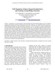
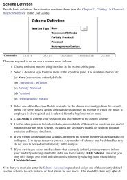
46-2 Mechanical VariablesFU xzyxdU x /dzFIGURE 46.1 System for defining Newtonian viscosity. When the upper plate is subjected to a force, the fluidbetween the plates is dragged in the direction of the force with a velocity of each layer that diminishes away fromthe upper plate. The reducing velocity eventually reaches zero at the lower plate boundary.top plate causes the fluid adjacent to the upper plate to move in the direction of F. The fluid adjacent tothe top plate is constrained by the no-slip boundary condition to move at the same speed as the plate.Similarly, the fluid next to the stationary bottom plate must be stationary. The motion of the top platethus causes the fluid to flow with a velocity profile across the liquid that decreases linearly from theupper to the lower plate, as shown in Figure 46.1. This arrangement is referred to as simple shear. Theapplied force is called a shear, and the force per unit area a shear stress. The resulting deformation rate ofthe fluid, or equivalently the velocity gradient dU x /dz, is called the shear strain rate, ġzx. The mathematicalexpression describing the viscous response of the system to the shear stress is simplytzxhdUxdU x= = hġ ⎛⎞zxhdz ⎝⎜separate and multiply from termdz ⎠⎟(46.1)whereτ zx , the shear stress, is the force per unit area exerted on the upper plate in the x-direction (andhence is equal to the force per unit area exerted by the fluid on the upper plate in the negativex-direction)dU x /dz is the gradient of the x-velocity in the z-direction in the fluid, that is, the shear strain rateη is the coefficient of viscosityNote that in general, the shear strain rate is more complex function of the fluid velocity-gradient tensor.In this case, because one is concerned with a shear force that produces the fluid motion, η is more specificallycalled the shear dynamic viscosity. In fluid mechanics, where the motion of a fluid is consideredwithout reference to force, it is common to define the kinematic viscosity, ν, which is simply given bynh= (46.2)rwhere ρ is the mass density of the fluid.The viscosity defined by Equation 46.1 is relevant only for laminar (i.e., layered or sheetlike) or streamlineflow as depicted in Figure 46.1, and it refers to the molecular viscosity or intrinsic viscosity. Themolecular viscosity is a property of the material that depends microscopically on interactions betweenindividual molecules and is manifested macroscopically as the fluid’s resistance to flow. When the flowis turbulent, small-scale turbulent vortices can contribute to the overall diffusion of momentum, resultingin an effective viscosity, sometimes called the eddy viscosity, that, depending on the Reynolds number,can be as much as 10 6 times larger than the intrinsic viscosity.Molecular viscosity is separated into shear viscosity and bulk or volume viscosity, η v , dependingon the type of strain involved. Shear viscosity is a measure of resistance to isochoric flow in a shearfield, whereas volume viscosity is a measure of resistance to volumetric flow in a 3D stress field.

Fluid Viscosity Measurement46-3For most liquids, including hydrogen bonded weakly associated or unassociated, and polymericliquids as well as liquid metals, η/η v ≈ 1, suggesting that shear and structural viscous mechanismsare closely related [1].The shear viscosity of most liquids decreases with temperature, which is opposite to what occursin gases. Under most conditions, including those relevant in engineering applications, viscositycan be considered to be independent of pressure, as temperature effects are very much larger. Inthe context of planetary interiors, however, the effects of pressure cannot be ignored, and pressurecontrols the viscosity to the extent that, depending on composition, it can cause fundamentalchanges in the molecular structure of the fluid that can result in an anomalous viscosity decreasewith increasing pressure [2].46.2 Newtonian and Non-Newtonian FluidsEquation 46.1 is known as Newton’s law of viscosity. If the viscosity throughout the fluid is independentof strain rate, then the fluid is said to be a Newtonian fluid. The constant of proportionality is calledthe coefficient of viscosity, and a plot of stress versus strain rate for Newtonian fluids yields a straightline with a slope of η, as shown by the solid line flow curve in Figure 46.2. Examples of Newtonian fluidsare pure, single-phase, unassociated gases; liquids; and solutions of low molecular weight such aswater. There is, however, a large group of fluids for which the viscosity is dependent on the strain rate.Such fluids are said to be non-Newtonian and their study is called rheology. In differentiating betweenNewtonian and non-Newtonian behavior, it is helpful to consider the time scale (as well as the normalstress differences and phase shift in dynamic testing) involved in the process of a liquid responding to ashear perturbation. In general, the shear strain rate g ̇ is more complex function of the second invariantof the fluid velocity-gradient tensor; however, in a simple shear flow, like on Figure 46.1, it reduces to thevelocity gradient, dU x /dz. Therefore, the time scale related to the applied shear perturbation about theequilibrium state is t s , where t s = ġ−1. A second time scale, t r , called the relaxation time, characterizesthe rate at which the relaxation of the strain in the fluid can be accomplished and is related to the timeit takes for a typical flow unit to move a distance equivalent to its mean diameter. For Newtonian water,t r ∼ 10 −12 s, and, because shear rates greater than 10 6 s −l are rare in practice, the time required for thefluid to respond to the strain perturbation in water is much less than the time scale of the perturbationitself (i.e., t r ≪ t s ). However, for non-Newtonian macromolecular liquids like polymeric liquids, for colloidaland fiber suspensions, and for pastes and emulsions, the long response times of large viscous flowunits (e.g., polymer molecules or aggregates of interacting particles) can easily make t r > t s . An exampleNon-NewtonianShear stressPseudoplastic materialsDilatant materialsNewtonian liquidsSlope ηStrain rateFIGURE 46.2Flow curves illustrating Newtonian and non-Newtonian fluid behavior.

46-4 Mechanical Variablesof a non-Newtonian fluid is liquid elemental sulfur, in which long chains (polymers) of up to 100,000sulfur atoms form flow units that are easily entangled, which bind the liquid in a “rigid-like” network.Another example of a well-known non-Newtonian fluid is tomato ketchup.With reference to Figure 46.2, Equation 46.1 can be written in a more general form:ġtxy()txy( ġ) = txy( ) + ∂ 0O( ġ20 + )∂ġ(46.3)Here τ xy (0) is a yield stress required for flow to start, the term proportional to g ̇ is the usual linearNewtonian term in limit of small strain rates, and the nonlinear term O( g ̇2 ) accounts for the nonlinearviscous response of some materials.For a Newtonian fluid, the initial stress at zero shear rate and the nonlinear function O( g ̇2 ) are bothnegligible (zero), so Equation 46.3 reduces to Equation 46.1, since ∂txy( 0)/∂ġ then equals η. For a non-Newtonian fluid, τ xy (0) may be zero but the nonlinear term O( g ̇2 ) is nonzero. This characterizes fluids inwhich shear stress varies nonlinearly with strain rate, as shown by the dashed-dotted and dashed flowcurves in Figure 46.2. The former type of fluid behavior is known as shear thickening or dilatancy, andan example is a concentrated suspension of cornstarch in water. The latter, much more common type offluid behavior is known as shear thinning or pseudoplasticity; cream, blood, most polymers, and liquidcement are all examples. Both behaviors result from particle or molecular reorientations or rearrangementsin the fluid that increase or decrease, respectively, the internal friction to shear. Non-Newtonianbehavior can also arise in fluids whose viscosity changes with time of applied shear stress. Fluids whoseviscosity increases over time when a shear stress is applied are called rheopectic. Conversely, liquidswhose viscosity decreases with time are called thixotropic fluids. Nondrip paint, which will not flowuntil a shear stress is applied by the paint brush for a sufficiently long time, is a common example of athixotropic fluid.Fluid deformation that is not recoverable after removal of the stress is typical of the purely viscousresponse. The other extreme response to an external stress is purely elastic and is characterized by anequilibrium deformation that is fully recovered on removal of the stress. There are an infinite numberof intermediate or combined viscous/elastic responses to external stress, which are grouped under thebehavior known as viscoelasticity. Fluids that behave elastically in some stress range require a limitingor yield stress before they will flow as a viscous fluid. A simple, empirical, constitutive equation oftenused for this type of rheological behavior is of the formnt = t + ġ h(46.4)yxypwhere τ y is the yield stress, η p is an apparent viscosity called the plastic viscosity, and the exponent nallows for a range of non-Newtonian responses: n = 1 describes pseudo-Newtonian behavior and iscalled a Bingham fluid; n < 1 describes shear thinning behavior; and n > 1 describes shear thickeningbehavior. Interested readers should consult [3–9] for further information on applied rheology.46.2.1 Dimensions and Units of ViscosityFrom Equation 43.1, the dimensions of dynamic viscosity are M L −1 T −1 , and the basic SI unit is thePascal second (Pa · s), where 1 Pa · s = 1 N s m −2 . The c.g.s. unit of dyn s cm −2 is the poise (P). Thedimensions of kinematic viscosity, from Equation 43.2, are L 2 T −1 , and the SI unit is m 2 s −1 . For mostpractical situations, this is usually too large and so the c.g.s. unit of cm 2 s −1 , or the stoke (St), ispreferred. Table 46.1 lists some common fluids and their shear dynamic viscosities at atmosphericpressure and 20°C.

Fluid Viscosity Measurement46-5TABLE 46.1 Shear Dynamic Viscosity of SomeCommon Fluids at 20°C and 1 atmFluidShear DynamicViscosity (Pa · s)Air1.8 × 10 −4Water1.0 × 10 −3Mercury1.6 × 10 −3Automotive engine oil (SAE 10W30) 1.3 × 10 −1Dish soap4.0 × 10 −1Corn syrup 6.046.3 Viscometer Types46.3.1 RheometerA viscometer (also called viscosimeter) is an instrument used to measure the viscosity of a fluid. Forliquids with viscosities, which vary with flow conditions, an instrument called a rheometer is used.Viscometers only measure under one flow condition. The instruments for viscosity measurementsare designed to determine “a fluid’s resistance to flow,” a fluid property defined earlier as viscosity.The fluid flow in a given instrument geometry defines the strain rates, and the corresponding stressesare the measure of resistance to flow. If strain rate or stress is set and controlled, then the other onewill, everything else being the same, depend on the fluid viscosity. If the flow is simple (one dimensional,if possible) such that the strain rate and stress can be determined accurately from the measuredquantities, the absolute dynamic viscosity can be determined; otherwise, the relative viscosity willbe established. For example, the fluid flow can be set by dragging the fluid with a sliding or rotatingsurface, or a body falling through the fluid, or by forcing the fluid (by external pressure or gravity) toflow through a fixed geometry, such as a capillary tube, annulus, a slit (between two parallel plates), ororifice. The corresponding resistance to flow is measured as the boundary force or torque or pressuredrop. The flow rate or efflux time represents the fluid flow for a set flow resistance, like pressure dropor gravity force. The viscometers are classified, depending on how the flow is initiated or maintained,as in Table 46.2.The basic principle of all viscometers is to provide as simple flow kinematics as possible, preferably 1D(isometric) flow, in order to determine the shear strain rate accurately, easily, and independent of fluidtype. The resistance to such flow is measured, and thereby the shearing stress is determined. The shearviscosity is then easily found as the ratio between the shearing stress and the corresponding shear strainrate. Practically, it is never possible to achieve desired 1D flow or ideal geometry, and a number of errors,listed in Table 46.3, can occur and need to be accounted for [4–8]. A sample list of manufacturers/distributors of commercial viscometers/rheometers is given in Table 46.4. There is no implied endorsementof any manufacturer on this list.46.3.2 Rotational Methods/Concentric CylindersThe main advantage of the rotational as compared to many other viscometers is its ability to operatecontinuously at a given shear rate, so that other steady-state measurements can be conveniently performed.That way, time dependency, if any, can be detected and determined. Also, subsequent measurementscan be made with the same instrument and sampled at different shear rates, temperature, etc.For these and other reasons, rotational viscometers are among the most widely used class of instrumentsfor rheological measurements.

46-6 Mechanical VariablesTABLE 46.2Type/GeometryViscometer/Rheometer Classification and Basic CharacteristicsBasic Characteristics/CommentsDrag flow types: Flow set by motion of instrument boundary/surface using external or gravity forceRotating concentric cylinders (Couette) Good for low viscosity, high shear rates; for R 2 /R 1 ≅ 1, see Figure 46.3;hard to clean thick fluidsRotating cone and plateHomogeneous shear, best for non-Newtonian fluids and normalstresses; need good alignment, problems with loadingand evaporationRotating parallel disksSimilar to cone and plate but inhomogeneous shear; shear varies withgap height, easy sample loadingSliding parallel platesHomogeneous shear, simple design, good for high viscosity; difficultloading and gap controlFalling body (ball, cylinder)Very simple, good for high temperature and pressure; need densityand special sensors for opaque fluids, not good for viscoelastic fluidsRising bubble oscillating bodySimilar to falling body viscometer; for transparent fluidsOscillating bodyNeeds instrument constant, good for low-viscous liquid metalsPressure flow types: Fluid set in motion in fixed instrument geometry by external or gravity pressureLong capillary (Poiseuille flow)Simple, very high shears and range but very inhomogeneous shear,bad for time dependency, and is time consumingOrifice/cup (short capillary)Very simple, reliable but not for absolute viscosity andnon-Newtonian fluidsSlit (parallel plates) pressure flowSimilar to capillary but difficult to cleanAxial annulus pressure flowSimilar to capillary, better shear uniformity but more complex,eccentricity problem and difficult to cleanOthers/miscellaneousUltrasonicGood for high-viscosity fluids, small sample volume, gives shear andvolume viscosity, and elastic property data; problems with surfacefinish and alignment, complicated data reductionSource: Adapted from Macosko, C. W., Rheology: Principles, Measurements, and Applications, VCH, New York, 1994.TABLE 46.3Error/EffectDifferent Causes of Viscometer/Rheometer ErrorsCause/CommentEnd/edge effectKinetic energy lossesSecondary flowNonideal geometryShear rate nonuniformityTemperature variation and viscous heatingTurbulenceSurface tensionElastic effectsMiscellaneous effectsEnergy losses at the fluid entrance and exit of main testgeometryLoss of pressure to kinetic energyEnergy loss due to unwanted secondary flow, vortices,etc.; increases with Reynolds numberDeviations from ideal shape, alignment, and finishImportant for non-Newtonian fluidsVariation in temperature, in time, and in space, influencesthe measured viscosityPartial and/or local turbulence often develops even at lowReynolds numbersDifference in interfacial tensionsStructural and fluid elastic effectsDepends on test specimen, melt fracture, thixotropy,rheopexy

Fluid Viscosity Measurement46-7TABLE 46.4 Viscometer/Rheometer Manufacturers and Distributors(for Measurement at 1 atm)A&D Engineering Co. Ltd Hydramotion PertenAmetek Kinematica AG Physica Messtechnik GmbHAnkersmid Lab Kittiwake RELAnton Parr Koehler Inst. Co., Inc. Reologica Instr.ATS Lamy Rheology Rheometric Scientific, Inc.Avenisense Lauda RheotecBartec Lemis Santam Eng. Energy Co. LtdBrookfield Eng. Labs, Inc. Malvern SI AnalyticsBYK Instr. Marimex So FraserCannon Inst. Co. Micro Motion Stanhope-SetaCeramic Instr. Nametre Co. T.A. Instruments, Inc.Cole-Palmer Inst. Co. Norcross TanakaDong Jin Inst. Corp. Orion Thermo ScientificFungilab Paar Physica USA, Inc. TMIGalvanic Applied Sciences, Inc. PAC Toyo Seiki Seisaku-Sho Ltd.Gottfert Werkstorf-Prufmaschinen GmbH Parker Weschler Instr.Note: All the previously mentioned manufacturers/distributors can be found on the Internet, alongwith their most recent contact information, product description, and, in some cases, pricing. A varietyof products using different viscosity measuring methods are available from this list.Concentric cylinder-type viscometers/rheometers are usually employed when absolute viscosity needsto be determined, which in turn requires knowledge of well-defined shear rate and shear stress data.Such instruments are available in different configurations and can be used for almost any fluid. Thereare models for low and high shear rates. More complete discussion on concentric cylinder viscometers/rheometers is given elsewhere [4–9]. In the Couette-type viscometer, the rotation of the outer cylinder,or cup, minimizes centrifugal forces, which cause Taylor vortices. The latter can be present in theSearle-type viscometer when the inner cylinder, or bob, rotates.Usually, the torque on the stationary cylinder and rotational velocity of the other cylinder are measuredfor determination of the shear stress and shear rate, respectively, which is needed for viscositycalculation. Once the torque, T, is measured, it is simple to describe the fluid shear stress at any pointwith radius r between the two cylinders, as shown in Figure 46.3:trqT()= r(46.5)22prLeIn Equation 46.5, L e = (L + L c ) is the effective length of the cylinder at which the torque is measured. Inaddition to the cylinder’s length L, it takes into account the end-effect correction L c [4–8].For a narrow gap between the cylinders (β = R 2 /R 1 ≅ 1), regardless of the fluid type, the velocity profilecan be approximated as linear, and the shear rate within the gap will be uniform:WRg () r ≅( R − R )2 1(46.6)whereΩ = (ω 2 − ω 1 ) is the relative rotational speedR – = (R 1 + R 2 )/2 is the mean radius of the inner (1) and outer (2) cylinders

46-8 Mechanical VariablesD 2 =2R 2TD 1 =2R 1OutercylinderLzFluidsamplerInnercylinderω 2FIGURE 46.3Concentric cylinders viscometer geometry.Actually, the shear rate profile across the gap between the cylinders depends on the relative rotationalspeed, radii, and the unknown fluid properties, which seems an “open-ended” enigma. The solution ofthis complex problem is given elsewhere [4–8] in the form of an infinite series and requires the slopeof a logarithmic plot of T as a function of Ω in the range of interest. Note that for a stationary innercylinder (ω 1 = 0), which is the usual case in practice, Ω becomes equal to ω 2 . However, there is a simplerprocedure [10] that has also been established by German standards [11]. For any fluid, including non-Newtonian fluids, there is a radius at which the shear rate is virtually independent of the fluid type fora given Ω. This radius, being a function of geometry only, is called the representative radius, R R , and isdetermined as the location corresponding to the so-called representative shear stress, τ R = (τ 1 + τ 2 )/2, theaverage of the stresses at the outer and inner cylinder interfaces with the fluid, that is,12 / 12 /2⎧ [ 2b] ⎫ ⎧ 2 ⎫RR = R1⎨ ⎬ = R22 ⎨ 2 ⎬⎩[ 1+b ] ⎭ ⎩[ 1+b ] ⎭(46.7)Since the shear rate at the representative radius is virtually independent on the fluid type (whetherNewtonian or non-Newtonian), the representative shear rate is simply calculated for Newtonian fluid(n = 1) and r = R R , according to [10]:ġ= ġ= wRr=RR22⎧[ b + 1]⎫⎨ 2 ⎬⎩[ b −1]⎭(46.8)The accuracy of the representative parameters depends on the geometry of the cylinders (β) and fluidtype (n).It is shown in [10] that, for an unrealistically wide range of fluid types (0.35 < n < 3.5) and cylindergeometries (β = 1–1.2), the maximum errors are less than 1%. Therefore, the error associated with therepresentative parameter concept is virtually negligible for practical measurements.

46-10 Mechanical Variableswhere R and θ 0 < 0.1 rad (≈6°) are the cone radius and angle, respectively. The viscosity is then easilycalculated asht qf [ 3Tq0]= =ġ32pWR(46.13)Inertia and secondary flow increase, while shear heating decreases the measured torque (T m ). For moredetails, see [4,5], and the torque correction is given asT m −= 1+ 6⋅10 4 Re 2(46.14)Twhere{ 2rWq [ ] } 0RRe =h(46.15)46.3.4 Parallel DisksThis geometry (Figure 46.5), which consists of a disk rotating in a cylindrical cavity, is similar to thecone-and-plate geometry, and many instruments permit the use of either one. However, the shear rateis no longer uniform but depends on radial distance from the axis of rotation and on the gap h, that is,ġr W() r = (46.16)hFor Newtonian fluids, after integration over the disk area, the torque can be expressed as a function ofviscosity, so that the latter can be determined ash = 2 Th[ pWR4 ](46.17)RUpperplateΩ, θFluidsamplehLowerplateTzrFIGURE 46.5Parallel disks viscometer geometry.

Fluid Viscosity Measurement46-1146.4 Pressure and Gravity Flow Methods46.4.1 Capillary ViscometersThe capillary viscometer is based on the fully developed laminar tube flow theory (Hagen–Poiseuilleflow) and is shown in Figure 46.6. The capillary tube length is many times larger than its small diameter,so that entrance flow is neglected or accounted for in more accurate measurement or for shorter tubes.The expression for the shear stress at the wall ist w = ⎡ ⎣ ⎢ΔPL⎤⎦⎥ ⋅ ⎡ ⎣ ⎢D4⎤⎦⎥(46.18)and2[ CrV]ΔP = ( P1− P2) + ( z1−z2)−2(46.19)where C ≅ 1.1, P, z, V = 4Q/[πD 2 ], and Q are correction factor, pressure, elevation, the mean flow velocity,and the fluid volume flow rate, respectively. The subscripts 1 and 2 refer to the inlet and outlet, respectively.The expression for the shear rate at the wall isg ̇⎧= [ 3 n + 1]⎫ 8V⎨ ⎬⎩ 4n⎭ ⋅ ⎧ ⎫⎨ ⎬⎭ (46.20)⎩ DSamplereservoirFluidsampleInletP 1 , z 1zCapillarytubeOutletP 2 , z 2VDrLFIGURE 46.6Capillary viscometer geometry.

46-12 Mechanical Variableswhere n = d[logτ w ]/d[log(8V/D)] is the slope of the measured log(τ w ) – log(8V/D) curve. Then, the viscosityis simply calculated asht ⎧ ⎫= = ⎨ ⎬g ⎩ + ⎭ ⋅ ⎧ 24w 4nΔPD⎫ ⎧ 4n⎫⎨ ⎬⎭ = ⎨ ⎬n ⎩ LV ⎩ n + ⎭ ⋅ ⎧[ΔPDp] ⎫̇⎨ ⎬[ 3 1] [ 32 ] [ 3 1]⎩ [ 128QL]⎭(46.21)Note that n = 1 for a Newtonian fluid, so the first term [4n/(3n + 1)] becomes unity and disappears fromthe earlier equations. The advantages of capillary over rotational viscometers are low cost, high accuracy(particularly with longer tubes), and the ability to achieve very high shear rates, even with high-viscositysamples. The main disadvantages are high residence time and variation of shear across the flow, whichcan change the structure of complex test fluids, as well as shear heating with high-viscosity samples.46.4.2 Glass Capillary ViscometersGlass capillary viscometers are very simple and inexpensive. Their geometry resembles a U-tube with atleast two reservoir bulbs connected to a capillary tube passage with inner diameter D. The fluid is drawnup into one bulb reservoir of known volume, V 0 , between etched marks. The efflux time, ∆t, is measuredfor that volume to flow through the capillary under gravity.From Equation 46.21 and taking into account that V 0 = (∆t)VD 2 π/4 and ∆P = ρg(z 1 − z 2 ), the kinematicviscosity can be expressed as a function of the efflux time only, with the last term, K/∆t, added toaccount for error correction, where K is a constant [7], that is,4h ⎧⎡4n⎤ pn = =r⎢⎣ +⎥⎦⋅ [ gz ( 1−z2) D] ⎫⎨⎬ ( Δt− KΔ t )(46.22)⎩ ( 3n1)128LVo⎭Note that for a given capillary viscometer and n ≅ 1, the curl-bracketed term is a constant. The lastcorrection term is negligible for a large capillary tube ratio, L/D, where kinematic viscosity becomeslinearly proportional to measured efflux time. Various kinds of commercial glass capillary viscometers,like Cannon–Fenske type or similar, can be purchased from scientific and/or supply stores. They arethe modified original Ostwald viscometer design in order to minimize certain undesirable effects, toincrease the viscosity range, or to meet specific requirements of the tested fluids, like opacity. Glasscapillary viscometers are often used for low-viscosity fluids.46.4.3 Orifice/Cup, Short Capillary: Saybolt ViscometerThe principle of these viscometers is similar to glass capillary viscometers, except that the flow througha short capillary (L/D ≪ 10) does not satisfy or even approximate the Hagen–Poiseuille, fully developed,pipe flow. The influences of entrance end effect and changing hydrostatic heads are considerable.The efflux time reading, ∆t, represents relative viscosity for comparison purposes and is expressed as“ viscometer seconds,” like the Saybolt seconds or Engler seconds or degrees. Although the conversionformula, similar to glass capillary viscometers, is used, the constants k and K in Equation 46.23 arepurely empirical and dependent on fluid types:h Kn = = kΔt−r Δt(46.23)where k = 0.00226, 0.0216, 0.073 and K = 1.95, 0.60, 0.0631, for Saybolt universal (∆t < 100 s), SayboltFurol (∆t > 40 s), and Engler viscometers, respectively [12,13]. Due to their simplicity, reliability, andlow cost, these viscometers are widely used for Newtonian fluids, in the oil and other industries, wheresimple correlations between the relative properties and desired results are needed. However, these viscometersare not suitable for absolute viscosity measurement nor for non-Newtonian fluids.

46-16 Mechanical Variables46.5.3 Falling Methods in Opaque LiquidsThe falling body methods described earlier have been extensively applied to transparent liquids whereoptical (often visual) observation of the falling body is possible. For opaque liquids, however, fallingbody methods require the use of some sensing technique to determine, often in situ, the position of thefalling body with respect to time. Techniques have varied, but they all have in common the ability todetect the body as it moves past the sensor. A recent study at high pressure [18] demonstrated that thecontrast in electric conductivity between a sphere and opaque liquid could be exploited to dynamicallysense the moving sphere if suitably placed electrodes penetrated the container walls as shown in theschematic diagram in Figure 46.9. References to other similar in situ techniques are given in [18].46.5.4 Rising Bubble/DropletFor many industrial processes, the rising bubble viscometer has been used as a method of comparing therelative viscosities of transparent liquids (such as varnish, lacquer, and beer) for decades. Although itsuse was widespread, the actual behavior of the bubble in a viscous liquid was not well understood untillong after the method was introduced [19]. The rising bubble method has been thought of as a derivativeof the falling sphere method; however, there are fundamental physical differences between the two. Themajor physical differences are as follows: (1) The density of the bubble is less that of the surroundingliquid, the compressibility of the bubble leads to a change in bubble volume depending on its rise positionin the fluid column, and (2) the bubble itself has some unique viscosity. Each of these differencesElectrodesdPassage of sphere throughthe electrode planesResistanceTimeFIGURE 46.9 Diagram of one type of apparatus used to determine the viscosity of opaque liquids in situ. Theelectrical signal from the passage of the falling sphere indicates the time to traverse a known distance (d) betweenthe two sensors.

Fluid Viscosity Measurement46-17can, and do, lead to significant and extremely complex rheological problems that have yet to be fullyexplained. If a bubble of gas or droplet of liquid with a radius, r b , and density, ρ′, is freely rising in someenclosing viscous liquid of density ρ, then the shear viscosity of the enclosing liquid is determined byr rh = ⎛ 2⎝ ⎜ 1 ⎞ [ 2grb( − ′)]e ⎠⎟9Ut(46.33)where( 2h+ 3 h′)e =3(h+ h′)(46.34)where η′ is the viscosity of the bubble. It must be noted that when η′ ≫ η, ε (as for solid spheres in afluid), ε = 1, which reduces Equation 46.33 to 46.25. For η′ ≪ η (as for gas bubbles in a fluid), ε becomes2/3, and the viscosity calculated by Equation 46.33 is 1.5 times greater than the viscosity calculated byEquation 46.25.During the rise, great care must be taken to avoid contamination of the bubble and its surface withimpurities in the surrounding liquid. Impurities can diffuse through the surface of the bubble andcombine with the fluid inside. Because the bubble has a low viscosity, the upward motion in a viscousmedium induces a drag on the bubble that is responsible for generating a circulatory motion within it.This motion can efficiently distribute impurities throughout the whole of the bubble, thereby changingits viscosity and density. Impurities left on the surface of the bubble can form a “skin” that cansignificantly affect the rise of the bubble, as the skin layer has its own density and viscosity that arenot included in Equation 46.33. These surface impurities also make a significant contribution to theinhomogeneous distribution of interfacial tension forces. A balance of these forces is crucial for theformation of a spherical bubble. The simplest method to minimize the earlier effects is to employ minutebubbles by introducing a specific volume of fluid (gas or liquid), with a syringe or other similar device,at the lower end of the cylindrical container. Very small bubbles behave like solid spheres, which makeinterfacial tension forces and internal fluid motion negligible.In all rising bubble viscometers, the bubble is assumed to be spherical. Experimental studies of theshapes of freely rising gas bubbles in a container of finite extent [20] have shown that (to 1% accuracy) abubble will form and retain a spherical shape if the ratio of the radius of the bubble to the radius of theconfining cylindrical container is less than 0.2. These studies have also demonstrated that the effect ofthe wall on the terminal velocity of a rising spherical bubble is to cause a large decrease (up to 39%) inthe observed velocity compared to the velocity measured within an unbounded medium. This impliesthat the walls of the container influence the velocity of the rising bubble more significantly than itsgeometry. In this method, end effects are known to be large. However, a rigorous, analytically or empiricallyderived correction factor has not yet appeared. To circumvent this, the ratio of container length tosphere diameter must be in the range of 10–100. As in other Stokesian methods, this allows the bubble’svelocity to be measured at locations that experience negligible end effects.Considering all of the earlier complications, the use of minute bubbles is the best approach to ensure aviscosity measurement that is least affected by both the liquid to be investigated and the container geometry.46.6 Oscillation MethodsOscillation methods are based on the measurement of viscous damping of oscillation within a fluidsample. Either the sample itself can be the wave carrying medium (acoustic method) or a separateoscillator can be used in forced oscillation or free decay mode (vibrating wire, transducer, or tuningfork methods). If a liquid is contained within a vessel suspended by some torsional system that is set

46-18 Mechanical Variablesin oscillation about its vertical axis, then the motion of the vessel will experience a gradual damping.In an ideal situation, the damping of the motion of the vessel arises purely as a result of the viscouscoupling of the liquid to the vessel and the viscous coupling between annular layers in the liquid. In anypractical situation, there are also frictional losses within the mechanical components of the suspensionsystem that contribute to damping and must be accounted for in the analysis of the measurements.From observations of the amplitudes and time periods of the resulting oscillations, a viscosity of theliquid can be calculated. A schematic diagram of the basic setup of the method is shown in Figure46.10. Following initial oscillatory excitation, a light source (such as a low-intensity laser) can be usedto measure the amplitudes and periods of the resulting oscillations by reflection of the mirror attachedto the suspension rod to give an accurate measure of the logarithmic decrement of the oscillations (δ)and the periods (T).Various working formulae have been derived that associate the oscillatory motion of a vessel ofradius r to the absolute viscosity of the liquid. The most reliable formula is the following equation for acylindrical vessel [21]:dh = ⎡ ⎣ ⎢ I ⎤3( prHZ)⎥⎦2⎡ 1 ⎤⎢⎣prT⎥⎦(46.35)where⎛ 1+r ⎞ZH a [( 32 / ) + ( 4r/ pH)] 1 [( 38 / ) + ( 9r/ 4H)]a=⎝⎜⎠⎟ 0 −+24p2p2(46.36)p = ⎛ ⎝ ⎜ pr ⎞hT⎠⎟12 /r(46.37)SuspensionfiberMirrorHρ2rFIGURE 46.10 Schematic diagram of the oscillating cup viscometer. Measurement of the logarithmic damping ofthe amplitude and period of vessel oscillation is used to determine the absolute shear viscosity of the liquid.

Fluid Viscosity Measurement46-19d 34 ⎠⎟ − ⎛ d ⎞p ⎝ ⎜ 32p⎠⎟2a 0 = 1 − ⎛ 2⎝ ⎜ ⎞(46.38)d4 ⎠⎟ + ⎛ d ⎞p ⎝ ⎜ 32p⎠⎟2a 2 = 1+ ⎛ 2⎝ ⎜ ⎞(46.39)whereI is the mass moment of inertia of the suspended systemρ is the density of the liquidA more practical expression of Equation 46.35 is obtained by introducing a number of simplifications.First, it is a reasonable assumption to consider δ to be small (on the order of 10 −2 to 10 −3 ). This reduces a 0and a 2 to values of 1 and −1, respectively. Second, the effects of friction from the suspension system andthe surrounding atmosphere can be experimentally determined and contained within a single parameteror instrument constant, δ 0 . This must then be subtracted from the measured δ. A common methodof obtaining δ 0 is to observe the logarithmic decrement of the system with an empty sample vessel andsubtract that value from the measured value of δ. With these modifications, Equation 46.35 becomeswhere12 / /( d − d ) ⎛ h ⎞ h h=r ⎝⎜ r ⎠⎟ − ⎛ ⎞⎝ ⎜ r ⎠⎟ + ⎛ 32⎡⎞ ⎤0⎢A B C⎝ ⎜ r ⎠⎟⎥(46.40)⎣⎢⎦⎥A = ⎛ /⎞ ⎡ r⎝ ⎜ I ⎠⎟ + ⎛ ⎝ ⎜ ⎞⎢1H ⎠⎟⎣ 4Hr Tp 32 3 1/2B = ⎛ r⎝ ⎜ p ⎞ ⎡I ⎠⎟ ⎛ ⎝ ⎜3⎞4 ⎤⎢ ⎠⎟ +⎣ 2 pH⎥⎦Hr 2TC = ⎛ /⎞ ⎡ r⎝ ⎜ I ⎠⎟ ⎛ ⎝ ⎜3⎞9 ⎤⎢ ⎠⎟ +2 ⎣ 8 4H⎥⎦HrT⎤⎥⎦p 12 32 /(46.41)(46.42)(46.43)It has been noted [22] that the analytical form of Equation 46.40 needs an empirically derived, instrument-constantcorrection factor (ζ) in order to agree with experimentally measured values of η. Thediscrepancy between the analytical form and the measured value arises as a result of the earlier assumptions.However, these assumptions are required as solutions of the differential equations of motion ofthis system are nontrivial. The correction factor is dependent on the materials, dimensions, and densitiesof each individual system but generally lies between the values of 1.0 and 1.08. The correction factor isobtained by comparing viscosity values of calibration materials determined by an individual system (withEquation 46.35) and viscosity values obtained by another reliable method such as the capillary method.With the earlier considerations taken into account, the final working Roscoe’s formula for the absoluteshear viscosity is12 / /( d − d ) ⎛ h ⎞ h h= zr ⎝⎜ r ⎠⎟ − ⎛ ⎞⎝ ⎜ r ⎠⎟ + ⎛ 32⎡⎞ ⎤0⎢A B C⎝ ⎜ r ⎠⎟⎥(46.44)⎣⎢⎦⎥

46-20 Mechanical VariablesThe oscillating cup method has been used and is best suited for use with low values of viscosity within therange of 10 −5 to 10 −2 Pa · s. Its simple closed design and use at high temperatures have made this methodvery popular for viscosity measurement of liquid metals.Perhaps the simplest version of the oscillation type of instrument is the vibrating-wire viscometer.Vibrating-wire viscometers are typically quite small and so require small quantities of fluid. They provideaccurate measurements but may require calibration using a known fluid. They can be used in quiteextreme conditions: the vibrating-wire viscometer was first used to measure the viscosity of liquidhelium at temperatures around 2 K [23,24]. Related instruments have been used at pressures in the GParange [25]. A viscometer based on a vibrating tuning fork, which is capable of accurate measurementsover a wide viscosity range (A & D Engineering), is available commercially.The theory of operation of the vibrating-wire viscometer has been described in detail in the literature[26]. It is based on the phenomenon of resonance. A wire (or more generally a thin beam) fixed at bothends will have a natural vibration frequency ω 0 determined by its length, physical properties, and tension.The vibration amplitude of the wire will be strongly peaked at that resonance frequency, and theheight and width of the resonant peak depending on the magnitude of the forces that damp the wire’smotion. For a vibrating wire immersed in a fluid, the width of the peak ∆ω or equivalently the qualityfactor Q = ω 0 /∆ω thus depends on viscosity, with higher viscosity leading to a smaller, broader peakand a lower Q. In a typical instrument, the vibrating wire sits in a uniform magnetic field produced bypermanent magnets. A small alternating current of angular frequency ω is passed through the wire, andthe resulting Lorentz forces cause the wire to vibrate at the same frequency. The voltage across the wirewill consist of a constant contribution due to the electrical impedance of the system plus an inducedemf that is proportional to the amplitude of the vibration. Vibrating-wire viscometers can operate in aforced mode, in which the wire is driven over a range of frequencies and the resonant peak measureddirectly, or in a transient mode, in which Q is determined from measurements of the decay rate of theoscillations following a short pulse of the driving current. In some configurations, the tension on thevibrating wire is applied by a mass suspended in the fluid. In this case, the instrument can be used tosimultaneously measure fluid density, since the tension and so the resonant frequency will depend onthe buoyant force acting on the mass.Several recent publications describe miniaturized versions of vibrating-object viscometers. Suchinstruments are of interest in applications ranging from the need for simple bedside measurements ofthe viscosity of blood, in which the quantity of fluid used must be minimized, to in situ measurementof viscosity in oil field reservoirs, in which the viscometer must withstand high temperatures and pressures.Very small vibrating beam and vibrating plate viscometers have been fabricated using microelectromechanicalsystem (MEMS) technology [27,28]. Smith et al. [29] describe a MEMS oscillating plateviscometer for human blood measurements. Dehestru et al. [30] discuss a vibrating-wire viscometerdesigned for oil field use. It has an internal volume of a few μL and is accurate to ±10% at pressures upto 24 MPa and temperatures up to 175°C.46.7 Acoustic MethodsViscosity plays an important role in the absorption of energy of an acoustic wave traveling through a liquid.By using ultrasonic waves (10 4 Hz < f < 10 8 Hz), the elastic, viscoelastic, and viscous response of a liquidcan be measured down to times as short as 10 ns. When the viscosity of the fluid is low, the resulting timescale for structural relaxation is shorter than the ultrasonic wave period, and the fluid is probed in therelaxed state. High-viscosity fluids subjected to ultrasonic wave trains respond as a stiff fluid because structuralequilibration due to the acoustic perturbation does not go to completion before the next wave cycle.Consequently, the fluid is said to be in an unrelaxed state that is characterized by dispersion (frequencydependentwave velocity) and elastic moduli that reflect a much stiffer liquid. The frequency dependence ofthe viscosity relative to some reference viscosity (η 0 ) at low frequency, η/η 0 , and of the absorption per wavelength,αλ, where α is the absorption coefficient of the liquid and λ is the wavelength of the compressional

Fluid Viscosity Measurement46-21Unrelaxed stateαλ η/η 0Relaxed stateFIGURE 46.11 Effects of liquid relaxation (relaxation frequency corresponds to ωτ = 1 where ω = 2πf) on relativeviscosity (upper) and absorption per wavelength (lower) in the relaxed elastic (ωτ < 1) and unrelaxed viscoelastic(ωτ > 1) regimes.1ωτwave, for a liquid with a single relaxation time, t, is shown in Figure 46.11. The maximum absorption perwavelength occurs at the relaxation frequency when ωτ = 1 and is accompanied by a step in η/η 0 , as well asin other properties such as velocity and compressibility. Depending on the application of the measuredproperties, it is important to determine if the liquid is in a relaxed or unrelaxed state.A schematic diagram of a typical apparatus for measuring viscosity by the ultrasonic method isshown in Figure 46.12. Mechanical vibrations in a piezoelectric transducer travel down one of the bufferrods (BR-1 in Figure 46.12) and into the liquid sample and are received by a similar transducer mountedon the other buffer rod, BR-2. In the fixed buffer rod configuration, once steady-state conditions havebeen reached, the applied signal is turned off quickly. The decay rate of the received and amplified signal,WavegeneratorGateBR-1SampleBR-2AmplifierabAmplitudeAmplitudeTimeMelt thicknessFIGURE 46.12 Schematic diagram of apparatus for liquid shear and volume viscosity determination by ultrasonicwave attenuation measurement showing the received signal amplitude through the exit buffer rod ( BR-2) using(a) a fixed buffer rod (BR-2) configuration and (b) an interferometric technique with moveable buffer rod.

46-22 Mechanical Variablesdisplayed on an oscilloscope on an amplitude versus time plot as shown in Figure 46.12a, gives a measureof α. The received amplitude decays as(A A e b a=c ) t0− + ′(46.45)whereA is the received decaying amplitudeA 0 is the input amplitudeb is an apparatus constant that depends on other losses in the system such as due to the transducerand container that can be evaluated by measuring the attenuation in a standard liquidc is the compressional wave velocity of the liquidt′ is timeAt low frequencies, the absorption coefficient is expressed in terms of volume and shear viscosity:⎛ h arhv + 4 ⎞ c⎝⎜⎠⎟ =3 2pf32 2(46.46)One of the earliest ultrasonic methods of measuring attenuation in liquids is based on acoustic interferometry[31]. Apart from the instrumentation needed to move and determine the position of one of the bufferrods accurately, the experimental apparatus is essentially the same as for the fixed buffer rod configuration[32]. The measurement, however, depends on the continuous acoustic wave interference of transmitted andreflected waves within the sample melt as one of the buffer rods is moved away from the other rod. Theattenuation is characterized by the decay of the maxima amplitude as a function of melt thickness as shownon the interferogram in Figure 46.12b. Determining a from the observed amplitude decrement involvesnumerical solution to a system of equations characterizing complex wave propagation [33]. The ideal conditionsrepresented in the theory do not account for conditions such as wave front curvature, buffer rod endnonparallelism, surface roughness, and misalignment. These problems can be addressed in the amplitudefitting stage, but they can be difficult to overcome. The interested reader is referred to [33] for further details.Ultrasonic methods have not been and are not likely to become the mainstay of fluid viscosity determinationsimply because they are more technically complicated than conventional viscometry techniques.And although ultrasonic viscometry supplies additional related elastic property data, its nichein viscometry is its capability of providing volume viscosity data. Since there is no other viscometer tomeasure η v , ultrasonic absorption measurements play a unique role in the study of volume viscosity.46.8 MicrorheologyOn the microscopic scale, viscosity is related to the phenomenon of diffusion. A small (i.e., micronsized) particle suspended in a viscous fluid such as water undergoes random motion as a result of thermalfluctuations in the forces acting on it. This is the well-known Brownian motion. Einstein showed ina famous 1905 [34] paper that the mean squared displacement 〈r 2 〉 of a particle undergoing Brownianmotion is given bywhereτ is the timed is the dimensionality of the motionThe angle brackets indicate an average over an ensemble of particles2r ( t)= 2dDt,(46.47)

Fluid Viscosity Measurement46-23D is the diffusion constant, which is related to the viscosity η of the fluid by the Stokes–Einstein equation:Herek B is the Boltzmann constantT is the absolute temperaturekT BD = (46.48)6ph aIf the radius a of the diffusing particles is known, these equations can be used to determine the viscosityfrom measurements of their mean squared displacement. In a viscoelastic fluid, the effects of elasticitymake the mean squared displacement grow more slowly than linearly. In this case, Equations 46.47 and46.48 can be generalized to relate the frequency-dependent viscous and elastic moduli to 〈r 2 〉. This isdiscussed in detail in Refs. [35–39].Several techniques collectively referred to as microrheology have been developed to make use ofthis relationship to measure viscosity or, more generally, the viscoelastic properties of fluids. The mostcommonly used of these will be discussed briefly in the following. The development and application ofmicrorheological techniques have been discussed in a number of review papers [35,40]. Microrheologycan be used to measure the properties of very small quantities of fluid and so is useful for characterizingexpensive or scarce fluids. On the other hand, while at least one commercial instrument is available,microrheology is still largely a research laboratory technique. For quantitative measurements ofthe bulk viscous and elastic moduli, the fluids being tested must be homogeneous on the scale of theparticle motion, since, if the fluid has small-scale structure, the local viscoelastic properties felt by thetracer particles can differ dramatically from the bulk properties. This is not an issue for most Newtonianfluids, but it can be for many complex fluids such as suspensions and gels.46.8.1 Particle-Tracking MicrorheologyParticle-tracking microrheology is based on direct imaging of small tracer particles undergoingBrownian motion in a fluid. This limits its application to fluids that are transparent or at least sufficientlyso that the positions of the tracer particles can be detected. The maximum viscosity that can bemeasured with particle tracking is limited by the requirement that the motion of the tracers must belarge enough to be detectable. This limit depends on the optical resolution of the microscope and imageanalysis procedure, as well as on the size of the tracers. For a typical experimental system, this limit ison the order of tens of Pa . s.Particle-tracking microrheology is done using a high-quality microscope fitted with a video camerainterfaced to a computer. Tracer particles are suspended in the fluid of interest, which is placed in asample holder and mounted on the stage of the microscope. Sample holders can be fabricated in anyvolume of fluid, but 10–100 μL is typical. The microscope must be focused on the center of the holder toavoid any influence of the walls on the motion of the tracer particles. The video camera records imagesof the tracer particles at a set frame rate, which are stored on the computer, and image analysis softwareis later used to reconstruct the particles’ trajectories and to calculate the mean squared displacement.To obtain good statistics in the data, the trajectories of many particles are tracked simultaneously, andthe concentration of tracers in the fluid is typically chosen to give about 50 particles in the microscope’sfield of view.The implementation details are discussed more fully elsewhere [35,40], but several points are worthmentioning. The tracer particles should be close in density to the fluid of interest so that they do notsettle over the course of the measurement. Polystyrene latex spheres with a density of 1.05 g cm –3can be obtained in a range of sizes and with a variety of chemical coatings and are typically used foraqueous solutions. It is important to ensure that the tracer particles do not interact chemically or

46-24 Mechanical VariablesAQ2electrostatically with the fluid being tested. Using bright-field microscopy, particles down to 0.5 μmin diameter can be tracked, while fluorescence microscopy can be used to track fluorescently dyedparticles as small as 0.1 μm in size. The shortest time over which the mean squared displacementcan be measured is limited by the video frame rate and the longest time by computer memory or thestability of the fluid.The stored video images of the diffusing particles must be analyzed to extract the trajectory of eachparticle and ultimately the mean squared displacement of the ensemble of particles. Several softwarepackages can be used to do this analysis. Particle-tracking software by Crocker and Grier [41] thatuses the IDL programming language is freely available [42] and has been used extensively. Thispackage has also been translated into MATLAB ® , and other image analysis software such as ImageJcould also be used. The image analysis involves filtering the images to remove background intensityvariations, identifying candidate particles by thresholding the images, determining their positionsto subpixel accuracy from the centroid of their brightness distribution, and finally reconstructingparticle trajectories by matching particles from one image to the next. Once the trajectories of allrecorded particles have been determined, their squared displacements are calculated and averaged.The viscosity, or the viscous and elastic moduli in the case of a non-Newtonian fluid, can then becalculated. Typically measurement uncertainties limit the observable mean squared displacement toabout 10 −4 μm 2 .An individual tracer particle moving in a viscoelastic fluid interacts hydrodynamically with othertracer particles. Two-particle microrheology exploits this fact by using correlations between the motionsof pairs of particles to obtain viscoelastic properties of the fluid on the scale of the separation betweenthe particles [43]. Two-particle microrheology gives moduli that are independent of the interactionsbetween the tracer particles and the material under study [43] and so gives the bulk properties evenin microscopically inhomogeneous fluids. Two-particle microrheology requires the same equipmentas described earlier. The difference comes in the data analysis, which, since it involves analyzing themotion of pairs of particles, requires much more data than in single-particle measurements. This techniquehas been used to study length-scale-dependent rheology in inhomogeneous materials such asactin networks [43], but for now it remains a research tool rather than a practical technique for routinemeasurements of material properties.46.8.2 Dynamic Light ScatteringA second microrheological technique uses dynamic light scattering to measure the mean squared displacementof tracer particles in the fluid. In this technique, incident laser light is scattered by particlessuspended in the fluid of interest. A photomultiplier mounted at an angle θ with respect to the incidentbeam measures the scattered light intensity, which fluctuates in time due to the random motion of thescattering particles. A digital correlator calculates the autocorrelation function of the scattered intensity,g 2 (τ), where τ is the time and g 2 is related to g 1 , the autocorrelation function of the scattered electricfield, which decays in time as(g e q / 6) ( ) r ( t )t = − ,(46.49)12 2where q = (4πn/λ)sin(θ/2), n is the refractive index of the fluid, and λ is the wavelength of the laserlight. The decay rate of g 1 (τ) thus gives the mean squared displacement of the tracer particles, fromwhich the viscosity or viscous and elastic moduli can be calculated using Equations 46.47 and46.48, as shown earlier. An example of data obtained using this technique is shown in Figure 46.13,where the mean squared displacement is plotted as a function of time for 110 nm polystyrenespheres in water.

Fluid Viscosity Measurement46-2510 –1 10 –410 –2 (μm 2 )10 –310 –410 –5Time (s)10 –3FIGURE 46.13 Mean squared displacement of 100 nm polystyrene sphere diffusion in water, measured usingdynamic light scattering. These data can be used to obtain the diffusion constant, from which the viscosity of thefluid can be determined. (From Yang, N. and deBruyn, J.R., unpublished.)A range of light scattering instruments, including laser, photodetector, and correlator, are availablecommercially, although many “black-box” scattering systems are intended for particle size determinationassuming a known viscosity. The tracer particles must again be neutrally buoyant in the fluid understudy, and their concentration must be low enough that the laser light is scattered at most once as itpasses through the sample holder. Typically a few milliliters of fluid is required, and the sample mustagain be transparent. Light scattering microrheology measures the viscoelastic properties of fluids atmuch higher frequencies than particle tracking, which is useful for characterizing complex fluids suchas polymer solutions.A related microrheological technique uses diffusing-wave spectroscopy. This is also a light scatteringtechnique but requires the light to be scattered many times in the sample, so that the light effectively diffusesthrough it. This requires a higher concentration of tracer particles. As shown earlier, the decay rateof the electric field autocorrelation function is related to the mean squared displacement of the tracerparticles, although the equations involved are slightly more complicated. Details are given in a numberof references. Diffusing-wave spectroscopy allows measurements at even higher frequencies than thesingle-scattering technique. An instrument that does microrheological measurements based on thistechnique is available commercially.46.9 High-Pressure RheologyMeasurement of viscosity of fluids at high pressures began with Bridgman [45]. Its primary interestwas to investigate liquids that would remain fluid at high pressures so they could be used as hydrostaticpressure-transmitting media in his experiments. Since that time, continued development ofhigh-pressure viscometry methods remained in the scientific research realm until recently. Overthe past decade, there has been increasing commercial and industrial interest in the application ofhigh-pressure technology in the processing of fluids. A wide range of foods, for example, are nowbeing processed using high-pressure technology principally as a nonthermal alternative for extendingshelf life. The technology also provides the food industry with a variety of new product developmentopportunities able to exploit the functional properties of ingredients such as hydrocolloids and proteins.High-pressure technology is proving increasingly attractive and beneficial in the destructionof microorganisms; activation and deactivation of enzymes; inactivation kinetics of both vegetative

46-26 Mechanical Variablesand pathogenic microorganisms; change of functional properties of biopolymers such as proteinsand polysaccharides used in foams, gels, and emulsions; and the control of phase change such as fatsolidification and ice melting point. The rheology of these fluids and soft solids is important to controlprocess function and speed. In other applications such as in the automotive industry, understandingthe high-pressure rheology of petroleum-based fuels is critical for the safe and efficient design andperformance of engines. High-pressure rheology has also been recognized as vital information forstudies of planetary interiors, where fluids of mainly silicate or metallic composition play significantroles in heat and mass flow and therefore fluid rheology is a pivotal parameter in controlling planetaryevolution.46.9.1 High-Pressure RheometryRheometry methods employed at high pressure are mainly based on traditional methods and can begrouped into four categories: concentric cylinder, capillary, oscillatory, and falling/rolling body. Thetheoretical treatment given earlier for each of these methods applies, but additional corrections maybe required for the container geometry effects due to the limited sample volumes imposed by the highpressureenvironment. The approaches to measure motion or stress in situ are often applied outside thehigh-pressure environment because of the high loads required and can involve detailed experimentalsetups. Also, depending on the pressure range, the equipment required to generate high pressure canbe much more elaborate than the equipment required to measure viscosity. Although there are severalhigh-pressure viscometers commercially available for use below a pressure of 1 GPa and examples arelisted in Table 46.5, measurement of viscosity at pressures above 1 GPa is carried out mainly in theresearch laboratory.Recent reviews of high-pressure viscosity measurement have appeared [46,47] and describe indetail the pressure devices and methods used up to ∼1 GPa. This appears to be the pressure limitof the concentric cylinder method because of the engineering challenges presented by the frictioneffects in rotating high-pressure seals and the difficulties in precise measurement of torque whenparts are subjected to high mechanical loads. Most high-pressure rotating systems use the Searleprinciple with a rotating inner cylinder and stationary outer cylinder. Methods of measuring theresulting shear stress include elastic torsion tubes, magnetic or inductive coupling, strain gaugeload cell, or variable torque induction motor. The capillary method is based on pressure-drivenflow. The pressure drop along the capillary is normally measured with pressure transducers, whichmust detect small pressure differences along the capillary on top of a large pressure signal arisingfrom the static high-pressure environment. High-pressure oscillation methods are based onthe measurement of viscous damping of an oscillator located within a pressurized fluid sample.Piezoelectric quartz crystals, which can operate at pressures exceeding 1 GPa, show a shift in thecrystal resonant frequency reflecting the mechanical shear impedance of the sample. A second wayto measure fluid viscosity is by observation of the free decay of a disk or wire-shaped oscillator.TABLE 46.5High-Pressure Viscometer/Rheometer ManufacturersManufacturers Maximum Pressure (Bars) MethodPSL Systemtechnik 1200 RotationalCambridge Viscosity, Inc. 1379 Oscillating piston/EMPAC 2040 Oscillating piston/EMChandler Engineering 2721 RotationalStony Brook Scientific, Inc. 4082 Falling needle/magneticF5 Technologie 5000 Torsional oscillation

Fluid Viscosity Measurement46-27A third way to measure viscosity using the oscillation method at high pressure is by passage oftransducer-generated and transducer-detected ultrasonic waves through the pressurized fluid. Theviscosity is calculated via the wave absorption coefficient of the sample, which is measured by signalattenuation at the receiving transducer.At pressures above 1 GPa, the falling/rolling body method is the preferred method although atleast one study of a capillary method employed to 6 GPa has been reported [48]. The simplicity andreliability of construction of components for the Stokesian method make it capable of providing viscositymeasurements at the highest pressures, where the sample fluid volume ranges from ∼10 −2 mm 3to a few mm 3 . In principle, viscosity can be measured with this method at pressures up to several 10’sof GPa and up to an order of magnitude greater than this using the diamond anvil cell. At such highpressures, high temperature is also required in order to melt the pressure-frozen liquid or becausethis range of pressures is mainly of interest to the Earth and planetary sciences and the relevant materialsto be studied have melting temperatures in excess of 1500°C. Such high temperatures requirejudicious selection of the material for the falling/rolling body to ensure solid-phase stability of thebody at the test conditions, chemical inertness of the body in the fluid, appropriate density contrastof the body and fluid, and ease of fabrication of the desired geometry. The velocimetry method useddepends on the body and fluid and on the observational access to the pressurized sample region.Since the diamond anvil cell has the great advantage of optical access through the diamond anvils,this is the method of choice for velocimetry of the moving body between two fiducial points. Inlarge-volume presses, which contain optically opaque components (usually ceramics and metals) inthe pressure cell, there are two main approaches to measuring the speed of the moving body. The firstinvolves allowing the body to move for a measured time in the pressurized fluid and then quenchingthe temperature to freeze the fluid, thereby capturing the body in position. Follow-up measurementof the body position is made by sectioning the recovered sample and measuring the distance thebody has moved. This is an effective method for measuring viscosities in the range of approximately10 −1 –10 5 Pa s if the density contrast of the body and fluid is chosen appropriately. A technique fortailoring the density of a probe sphere, by cladding a metallic core sphere with a refractory mantleto make a composite sphere [49], allows for adjustment of the fall time of the body to within acceptableranges considering the fluid density and its expected viscosity. However, for measuring muchlower viscosities, the control on quenching the temperature and accurate determination of the bodystart/stop position are inadequate, and therefore, in situ velocimetry methods are required. Manyin situ velocimetry methods have been devised based on the following with either in situ or ex situcomponents for detection: electromagnetic induction using a two-coil external arrangement and anelectrically conducting body in a nonconducting fluid, detecting passage of an insulating body movingthrough two electrodes placed in a metallic fluid by measuring electrical resistance of the fluid,detecting passage of a weakly radioactive body such as a 60 Co sphere sensed by an external scintillationcounter, and x-ray radiographic imaging of a body with sufficient absorption x-ray contrastwith the fluid. Over the last decade, the last method has become the method of choice for accuratehigh-pressure viscometry at pressures above 1 GPa [50] on low-viscosity fluids and is described infurther detail.Experiments to measure the viscosity of a fluid at high temperatures and at pressures above 1 GPaare frequently carried out using the x-ray radiography imaging technique in real time at a synchrotronfacility. The high photon flux at a synchrotron is needed in order to produce images of sufficient qualityand at high enough frequency (or ideally a movie) at various positions during travel of the body inorder to derive a velocity. The x-ray radiographic technique images the pressurized region according tothe relative x-ray attenuation coefficients of the experimental materials. A diagram of the experimentalimaging setup for a high-pressure Stokesian viscometry measurement using synchrotron x-ray radiography,the resultant sequence of time lapse images, and the sphere displacement and velocity data for afalling composite sphere is shown in Figure 46.14.

46-28 Mechanical VariablesSecond stage anvil (WC)CCD cameraFirst stage anvilSlit26 mmWhite beam(a)High-pressure cellFluorescence screenMirror(b)51.641.2Velocity (mm s –1 )320.80.4Distance (mm)10.0(c)00.0 0.1 0.2 0.3 0.4Time (s)0.5 0.6FIGURE 46.14 (a) Synchrotron x-ray radiography setup for a high-pressure Stokesian viscometry measurement[51]. (b) Synchrotron radiographic images of a Pt core—ruby mantle composite sphere falling in liquid Fe–29 wt% S at2.6 GPa and 1373 K. Images are separated in time by 62 ms [52]. (c) Distance and velocity of falling composite sphereversus time in Fe–29 wt% S liquid, at 2.6 GPa and 1373 K. Dashed line is terminal velocity [52].

Fluid Viscosity Measurement46-29References1. T. A. Litovitz and C. M. Davis, Structural and shear relaxation in liquids: In: W. P. Mason (Ed.),Physical Acoustics: Principles and Methods, Vol. II, Part A, Properties of Gases, Liquids and Solutions,New York: Academic Press, 1965, pp. 281–349.2. Y. Bottinga and P. Richet, Silicate melts: The “anomalous” pressure dependence of the viscosity,Geochim. Cosmochim. Acta, 59, 2725–2731, 1995.3. J. Ferguson and Z. Kemblowski, Applied Fluid Rheology, New York: Elsevier, 1991.4. R. W. Whorlow, Rheological Techniques, 2nd edn., New York: Ellis Horwood, 1992.5. K. Walters, Rheometry, London: Chapman and Hall, 1975.6. J. M. Dealy, Rheometers for Molten Plastics, New York: Van Nostrand Reinhold, 1982.7. J. R. Van Wazer, J. W. Lyons, K. Y. Kim, and R. E. Colwell, Viscosity and Flow Measurement, New York:Interscience, 1963.8. C. W. Macosko, Rheology: Principles, Measurements, and Applications, New York: VCH, 1994.9. W. A. Wakeham, A. Nagashima, and J. V. Sengers (Eds.), Measurement of the Transport Properties ofFluids, Oxford, U.K.: Blackwell Scientific, 1991.10. J. A. Himenez and M. Kostic, A novel computerized viscometer/rheometer, Rev. Sci. Instrum., 65(1),229–241, 1994.11. DIN 53018 (Parts 1 and 2), 53019, German National Standards.12. Marks’ Standard Handbooks for Mechanical Engineers, New York: McGraw-Hill, 1978.13. ASTM D445-71 standard.14. W. D. Kingery, Viscosity in Property Measurements at High Temperatures, New York: John Wiley &Sons, 1959.15. H. Faxen, Die Bewegung einer Starren Kugel Langs der Achsee eines mit Zaher Flussigkeit GefulltenRohres: Arkiv for Matematik, Astronomi och Fysik, 27(17), 1–28, 1923.16. F. Gui and T. F. Irvine, Jr., Theoretical and experimental study of the falling cylinder viscometer, Int.J. Heat Mass Transfer, 37(1), 41–50, 1994.17. N. A. Park and T. F. Irvine, Jr., Falling cylinder viscometer end correction factor, Rev. Sci. Instrum.,66(7), 3982–3984, 1995.18. G. E. LeBlanc and R. A. Secco, High pressure stokes’ viscometry: A new in-situ technique for spherevelocity determination, Rev. Sci. Instrum., 66(10), 5015–5018, 1995.19. R. Clift, J. R. Grace, and M. E. Weber, Bubbles, Drops, and Particles, San Diego: Academic Press, 1978.20. M. Coutanceau and P. Thizon, Wall effect on the bubble behavior in highly viscous liquids, J. FluidMech., 107, 339–373, 1981.21. R. Roscoe, Viscosity determination by the oscillating vessel method I: Theoretical considerations,Proc. Phys. Soc., 72, 576–584, 1958.22. T. Iida and R. I. L. Guthrie, The Physical Properties of Liquid Metals, Oxford, UK: Clarendon Press, 1988.23. J. T. Tough, W. D. McCormick, and J. G. Dash, Viscosity of liquid He II, Phys. Rev., 132, 2373–2378, 1963.24. J. T. Tough, W. D. McCormick, and J. G. Dash, Vibrating wire viscometer, Rev. Sci. Instrum., 35,1345–1348, 1964.25. P. S. vander Gulik, R. Mostert, and H. R. vanden Berg, The viscosity of methane at 273 K up to 1 GPa,Fluid Phase Equil., 79, 301–311, 1992.26. T. Retsina, S. M. Richardson, and W. A. Wakeham, The theory of a vibrating-rod viscometer Appl.Sci. Res., 43, 325–346, 1987.27. C. Riesch, E. K. Reichel, A. Jachimowicz, J. Schalko, P. Hudek, B. Jakoby, and F. Keplinger, A suspendedplate viscosity sensor featuring in-plane vibration and piezoresistive readout, J. Micromech.Microeng., 19, 075010 1–10, 2009.28. Y. Zhao, S. Li, A. Davidson, B. Yang, Q. Wang, and Q. Lin, A MEMS viscometric sensor for continuousglucose monitoring, J. Micromech. Microeng., 17, 2528–2537, 2007.AQ3AQ4

46-30 Mechanical Variables29. P. D. Smith, R. C. D. Young, and C. R. Chatwin, A MEMS viscometer for unadulterated humanblood, Measurement, 43, 144–151, 2010.30. G. Dehestru, M. Leman, J. Jundt, P. Dryden, M. Sullivan, and C. Harrison, A microfluidic vibratingwire viscometer for operation at high pressure and high temperature, Rev. Sci. Instrum., 82, 0351131–5, 2011.31. H. J. McSkimin, Ultrasonic methods for measuring the mechanical properties of liquids and solids,In: W. P. Mason (Ed.), Physical Acoustics: Principles and Methods, Vol. I, Part A, Properties of Gases,Liquids and Solutions, New York: Academic Press, 1964, pp. 271–334.32. P. Nasch, M. H. Manghnani, and R. A. Secco, A modified ultrasonic interferometer for sound velocitymeasurements in molten metals and alloys, Rev. Sci. Instrum., 65, 682–688, 1994.33. K. W. Katahara, C. S. Rai, M. H. Manghnani, and J. Balogh, An interferometric technique for measuringvelocity and attenuation in molten rocks, J. Geophys. Res., 86, 11779–11786, 1981.34. A. Einstein, Ueberdievondermolekularkinetis chentheoriederwaermegefordertebewegung voninruhendenfluessigkeitensuspendiertenteilchen,Ann. Phys., 17, 549–560, 1905.35. M. L. Gardel, M. T. Valentine, and D. A. Weitz, Microrheology, In: K. Breuer (Ed.), MicroscaleDiagnostic Techniques, New York: Springer, 2005.36. T. G. Mason and D. A. Weitz, Optical measurements of frequency-dependent linear viscoelasticmoduli of complex fluids, Phys. Rev. Lett., 74, 1250–1253, 1995.37. T. G. Mason, Estimating the viscoelastic moduli of complex fluids using the generalized Stokes–Einstein equation, Rheol. Acta., 39, 371–378, 2000.38. A. J. Levine and T. C. Lubensky, One- and two-particle microrheology, Phys. Rev. Lett., 85, 1774–1777, 2000.39. A. J. Levine and T. C. Lubensky, Response function of a sphere in a viscoelastic two-fluid medium,Phys. Rev. E, 63, 041510 1–12, 2001.40. T. A. Waigh, Microrheology of complex fluids, Rep. Prog. Phys., 68, 685–742, 2005.41. J. Crocker and D. G. Grier, Methods of digital video microscopy for colloidal studies, J. ColloidInterface Sci., 179, 298–310, 1996.42. J. Crocker and E. Weeks, Particle tracking using IDL, 1996, http://www.physics.emory.edu/∼weeks/idl/43. J. C. Crocker, M. T. Valentine, E. R. Weeks, T. Gisler, P. D. Kaplan, A. G. Yodh, and D. A. Weitz, Twopointmicrorheology of inhomogeneous soft materials, Phys. Rev. Lett., 85, 888–891, 2000.44. N. Yang and J. R. deBruyn, unpublished.45. P. W. Bridgman, The viscosity of liquids under pressure, Proc. Natl. Acad. Sci., 11, 603–606, 1925.46. L. Kulisiewicz and A. Delgado, High pressure rheological measurement methods: A review, Appl.Rheol., 20, 13018, 201047. C. J. Schaschke, High pressure viscosity measurement with falling body type viscometers, Int. Rev.Chem. Eng., 2, 564–576, 2010.48. J. D. Barnett and C. D. Bosco, Viscosity measurements on liquids to pressures of 60 kbar, J. Appl.Phys., 40, 3144–3150, 1969.49. R. A. Secco, R. F. Tucker, S. P. Balog, and M. D. Rutter, Tailoring sphere density for high pressurephysical property measurements on liquids, Rev. Sci. Instrum., 71, 2114–2116, 2001.50. T. Uchida, Y. Wang, M. L. Rivers, S. R. Sutton, D. J. Weidner, M. T. Vaughan, J. Chen, B. Li, R. A. Secco,M. D. Rutter, and H. Liu, A large-volume press facility at the Advanced Photon Source: Diffractionand imaging studies on materials relevant to the cores of planetary bodies, J. Phys. Condens. Matter.,14, 11517–11523, 2002.51. K. Funakoshi, A. Suzuki, and H. Terasaki, In situ viscosity measurements of albite melt under highpressure, J. Phys. Condens. Matter., 14, 11343–11347, 2002.52. R. A. Secco, M. D. Rutter, S. P. Balog, H. Liu, D. C. Rubie, T. Uchida, D. Frost, Y. Wang, M. Rivers,and S. R. Sutton, Viscosity and density of Fe–S liquids at high pressures, J. Phys. Condens. Matter.,14, 11325–11330, 2002.

Fluid Viscosity Measurement46-31Further InformationBrooks, R. F., Dinsdale, A. T., and Quested, P. N., The measurement of viscosity of alloys—A review ofmethods, data and models, Meas. Sci. Technol., 16, 354–362, 2005, a review of methods used to measureviscosity of liquid metals including methods adaptable to “in plant” measurement of fluid flowin metallurgical industrial processes.Hou, Y. Y. and Kassim, H. O., Instrument techniques for rheometry, Rev. Sci. Instrum., 76. 101101, 2005, areview of some of the latest advances in rheology measuring techniques including new approachesto conventional velocimetry (e.g., nuclear magnetic resonance, ultrasound pulse Doppler mapping)as well as other techniques that are important for industrial processes (e.g., extensional rheometryand interfacial rheometry).O’Neill, M. E. and Chorlton, F., Viscous and Compressible Fluid Dynamics, Chichester, U.K.: Ellis Horwood,1989, mathematical methods and techniques and theoretical description of flows of Newtonianincompressible and ideal compressible fluids.Ryan, M. P. and Blevins, J. Y. K., The viscosity of synthetic and natural silicate melts and glasses at hightemperatures and 1 bar (10 5 Pascals) pressure and at higher pressures, U.S. Geological Survey Bulletin1764, Denver, CO, 1987, p. 563, an extensive compilation of viscosity data in tabular and graphicformat and the main techniques used to measure shear viscosity.Van Wazer, J. R., Lyons, J. W., Kim, K. Y., and Colwell, R. E., Viscosity and Flow Measurement: A LaboratoryHandbook of Rheology, New York: Interscience Publishers, Division of John Wiley & Sons, 1963,A comprehensive overview of viscometer types and simple laboratory measurements of viscosityfor liquids.Author Queries[AQ1] Please check if the given order of authors is correct.[AQ2] Please provide the expansion of the acronym “IDL,” if appropriate.[AQ3] Please update Refs. [13,44].[AQ4] Please provide in-text citation for Ref. 14.