Non-local Models of Stiffness and Damping - Michael I Friswell

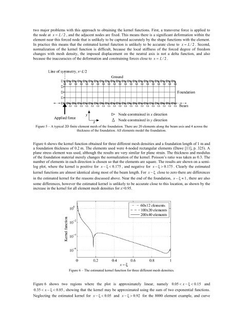
two major problems with this approach to obtaining the kernel functions. First, a transverse force is applied to
the node at x = L /2, and the adjacent nodes are fixed. This means there is a significant deformation within the
element near this forced node that is unlikely to be captured accurately by the shape functions with the element.
In practice this means that the estimated kernel function is unlikely to be accurate close to x = L /2. Second,
normalization of the kernel function is difficult, because the local stiffness of the forced degree of freedom
changes with mesh density, the imposed displacement on the neutral axis is not a delta function, and also
because the inaccuracies of the deformation and constraining forces close to x = L /2.
Figure 5 – A typical 2D finite element mesh of the foundation. There are 20 elements along the beam axis and 4 across the
thickness of the foundation. All elements model the foundation.
Figure 6 shows the kernel function obtained for three different mesh densities and a foundation length of 1 m and
a foundation thickness of 0.2 m. The elements used were 4-noded rectangular elements (Dawe [11], p. 325). A
plane stress element was used, although the results are very similar for plane strain. The thickness and modulus
of the foundation material merely changes the normalization of the kernel. Poisson’s ratio was taken as 0.3. The
number of elements in each direction is chosen so that the elements are square. The results are shown on a semilog
plot, where the kernel is positive for x −ξ< 0.175 , and negative for x −ξ> 0.175 . Clearly the estimated
kernel functions are almost identical along most of the beam length. For x −ξ close to zero there are differences
in the estimated kernel for the reasons discussed above. Near the end of the foundation, x − ξ ≈ 1 , there are also
some differences, however the estimated kernel is unlikely to be accurate close to this location, as shown by the
increase in the kernel for all element mesh densities for x>0.95.
Figure 6 – The estimated kernel function for three different mesh densities.
Figure 6 shows two regions where the plot is approximately linear, namely 0.05 < x −ξ < 0.15 and
0.35 < x −ξ < 0.85 , showing that the kernel may be approximated using the sum of two exponential functions.
Neglecting the estimated kernel for x − ξ < 0.05 and x −ξ> 0.92 for the 8000 element example, and curve