Non-local Models of Stiffness and Damping - Michael I Friswell
Non-local Models of Stiffness and Damping - Michael I Friswell
Non-local Models of Stiffness and Damping - Michael I Friswell

Create successful ePaper yourself
Turn your PDF publications into a flip-book with our unique Google optimized e-Paper software.
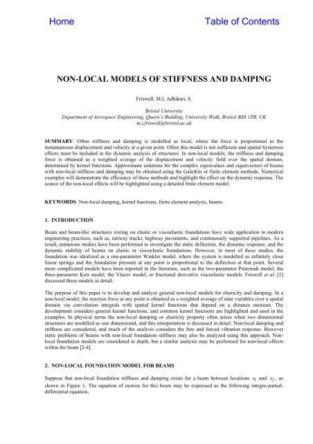
NON-LOCAL MODELS OF STIFFNESS AND DAMPING<br />
<strong>Friswell</strong>, M.I, Adhikari, S.<br />
Bristol University<br />
Department <strong>of</strong> Aerospace Engineering, Queen’s Building, University Walk, Bristol BS8 1TR, UK<br />
m.i.friswell@bristol.ac.uk<br />
SUMMARY: Often stiffness <strong>and</strong> damping is modelled as <strong>local</strong>, where the force is proportional to the<br />
instantaneous displacement <strong>and</strong> velocity at a given point. Often this model is not sufficient <strong>and</strong> spatial hysteresis<br />
effects must be included in the dynamic analysis <strong>of</strong> structures. In non-<strong>local</strong> models, the stiffness <strong>and</strong> damping<br />
force is obtained as a weighted average <strong>of</strong> the displacement <strong>and</strong> velocity field over the spatial domain,<br />
determined by kernel functions. Approximate solutions for the complex eigenvalues <strong>and</strong> eigenvectors <strong>of</strong> beams<br />
with non-<strong>local</strong> stiffness <strong>and</strong> damping may be obtained using the Galerkin or finite element methods. Numerical<br />
examples will demonstrate the efficiency <strong>of</strong> these methods <strong>and</strong> highlight the effect on the dynamic response. The<br />
source <strong>of</strong> the non-<strong>local</strong> effects will be highlighted using a detailed finite element model.<br />
KEYWORDS: <strong>Non</strong>-<strong>local</strong> damping, kernel functions, finite element analysis, beams.<br />
1. INTRODUCTION<br />
Beam <strong>and</strong> beam-like structures resting on elastic or viscoelastic foundations have wide application in modern<br />
engineering practices, such as, railway tracks, highway pavements, <strong>and</strong> continuously supported pipelines. As a<br />
result, numerous studies have been performed to investigate the static deflection, the dynamic response, <strong>and</strong> the<br />
dynamic stability <strong>of</strong> beams on elastic or viscoelastic foundations. However, in most <strong>of</strong> these studies, the<br />
foundation was idealized as a one-parameter Winkler model, where the system is modelled as infinitely close<br />
linear springs <strong>and</strong> the foundation pressure at any point is proportional to the deflection at that point. Several<br />
more complicated models have been reported in the literature, such as the two-parameter Pasternak model, the<br />
three-parameter Kerr model, the Vlasov model, or fractional derivative viscoelastic models. <strong>Friswell</strong> et al. [1]<br />
discussed these models in detail.<br />
The purpose <strong>of</strong> this paper is to develop <strong>and</strong> analyze general non-<strong>local</strong> models for elasticity <strong>and</strong> damping. In a<br />
non-<strong>local</strong> model, the reaction force at any point is obtained as a weighted average <strong>of</strong> state variables over a spatial<br />
domain via convolution integrals with spatial kernel functions that depend on a distance measure. The<br />
development considers general kernel functions, <strong>and</strong> common kernel functions are highlighted <strong>and</strong> used in the<br />
examples. In physical terms the non-<strong>local</strong> damping or elasticity property <strong>of</strong>ten arises when two dimensional<br />
structures are modelled as one dimensional, <strong>and</strong> this interpretation is discussed in detail. <strong>Non</strong>-<strong>local</strong> damping <strong>and</strong><br />
stiffness are considered, <strong>and</strong> much <strong>of</strong> the analysis considers the free <strong>and</strong> forced vibration response. However<br />
static problems <strong>of</strong> beams with non-<strong>local</strong> foundation stiffness may also be analyzed using this approach. <strong>Non</strong><strong>local</strong><br />
foundation models are considered in depth, but a similar analysis may be performed for non-<strong>local</strong> effects<br />
within the beam [2-4].<br />
2. NON-LOCAL FOUNDATION MODEL FOR BEAMS<br />
Suppose that non-<strong>local</strong> foundation stiffness <strong>and</strong> damping exists for a beam between locations 1 x <strong>and</strong> 2 x , as<br />
shown in Figure 1. The equation <strong>of</strong> motion for this beam may be expressed as the following integro-partialdifferential<br />
equation,
( )<br />
( )<br />
2<br />
2 2<br />
∂ ⎛ ∂ wxt , ⎞ ∂ wxt ,<br />
EI ( x)<br />
A( x)<br />
Q<br />
2<br />
⎜<br />
2<br />
⎟ +ρ +<br />
2 NE x + QND<br />
x = f x t<br />
∂x ⎝ ∂x ⎠ ∂t<br />
( ) ( ) ( , )<br />
(1)<br />
where EI ( x ) is the bending stiffness <strong>of</strong> the beam, ρ A( x)<br />
is the mass per unit length <strong>of</strong> the beam, ( , )<br />
transverse displacement, <strong>and</strong> f ( xt , ) is the distributed external force. Q ( x ) <strong>and</strong> Q ( )<br />
wxt is the<br />
NE<br />
ND x are the forces due<br />
to the foundation elasticity <strong>and</strong> damping, which are assumed to be non-<strong>local</strong>. These forces are given by<br />
x<br />
QNE<br />
x t C x w t<br />
x1<br />
2<br />
2<br />
( , ) = ∫ E ( , ξ) ( ξ, ) dξ<br />
<strong>and</strong> QND<br />
( x t) CD<br />
( x t )<br />
x<br />
x1<br />
( ξ,<br />
τ)<br />
t<br />
∂w<br />
, = , ξ, −τ dτdξ<br />
−∞<br />
∂t<br />
∫ ∫ . (2)<br />
CE ( x , ξ ) <strong>and</strong> CD<br />
( x, ξ, t−τ ) are the one-dimensional kernel functions for the elasticity <strong>and</strong> damping<br />
respectively, defined over the spatial sub domain ( x1,<br />
x 2)<br />
. The appropriate boundary conditions must be<br />
satisfied at x = 0 <strong>and</strong> x = L .<br />
Figure 1 – A beam with a partial non-<strong>local</strong> foundation.<br />
2.1. Typical Kernel Functions<br />
The general kernel function allows for both time <strong>and</strong> spatial hysteresis, representing a non-<strong>local</strong> viscoelastic<br />
damping model. If the kernel functions are assumed to be separable in space <strong>and</strong> time, then C ( x, ξ, t −τ ) <strong>and</strong><br />
CD ( x , ξ , t−τ ) are <strong>of</strong> the form<br />
( , ξ ) = ( ) ( −ξ ) <strong>and</strong> C ( x, , t ) H ( x) c ( x ) g( t )<br />
CE<br />
x H x cE<br />
x<br />
D<br />
ξ −τ = D −ξ −τ (3)<br />
where H ( x ) indicates the presence <strong>of</strong> the foundation, c( x− ξ ) is the spatial kernel <strong>and</strong> g ( t ) is the time kernel.<br />
The spatial kernel functions, c( x−ξ ) , where the subscript E or D is implicitly assumed, are usually normalised<br />
to satisfy the condition<br />
∞<br />
−∞<br />
∫ c( x)dx<br />
= 1. (4)<br />
Common choices for the spatial kernel function, c( x− ξ ) , are an exponential decay,<br />
or an error function,<br />
α −α x−ξ<br />
c( x−ξ ) = e , (5)<br />
2<br />
E<br />
( )<br />
c x−ξ =<br />
α<br />
2π<br />
e<br />
α<br />
2 −<br />
2<br />
( x−ξ) 2<br />
, (6)<br />
where α is the characteristic parameter <strong>of</strong> the non-<strong>local</strong> effect. Notice that, c( x−ξ) → 0 when α→∞ <strong>and</strong><br />
x ≠ ξ , so that c( x−ξ) →δ( x−ξ ) , which is the model for <strong>local</strong> elasticity or damping. Thus, 1/α is called the<br />
influence distance.
Often the time kernel function, g () t , is assumed to be <strong>of</strong> the form<br />
M<br />
g()<br />
t = g r<br />
r μr<br />
e −μ t<br />
r=<br />
1<br />
∑ (7)<br />
where μ r are the relaxation constants <strong>of</strong> the viscoelastic material, that may be determined by curve fitting <strong>of</strong> the<br />
measured mechanical properties <strong>of</strong> the material. Other forms <strong>of</strong> g(t), such as the GHM model [5,6] may also be<br />
analysed using the proposed method. The fractional derivative model [7] may also be used, but is better<br />
described in the Laplace domain. These models are not considered further as the spatial hysteresis is the main<br />
concern <strong>of</strong> this paper.<br />
2.2. Finite Element Analysis <strong>of</strong> Beams with <strong>Non</strong>-<strong>local</strong> Foundations<br />
For simple beam structures methods such as the transfer function method [3] or the Galerkin approach [4] may<br />
be used. For the analysis <strong>of</strong> general beam structures, <strong>Friswell</strong> et al. [1] introduced the non-<strong>local</strong> effects into a<br />
finite element analysis. Generally the approach adopted when developing models using finite element analysis is<br />
to approximate the deformation within an element using nodal values <strong>of</strong> displacement <strong>and</strong> rotation. The kinetic<br />
<strong>and</strong> strain energy for each element is then computed <strong>and</strong> the contributions <strong>of</strong> each element added together to<br />
obtain a global model <strong>of</strong> the structure. The damping matrix is obtained is a similar way using the dissipation<br />
function. One key aspect <strong>of</strong> finite element analysis is that the energy contribution from each element only<br />
depends on the displacements <strong>and</strong> rotations at the nodes associated with that element. Clearly for non-<strong>local</strong><br />
elasticity this will not be the case, although the form <strong>of</strong> the exponential kernel function does lead to considerable<br />
simplification [1].<br />
A st<strong>and</strong>ard beam element is modelled using two nodes (at the ends <strong>of</strong> the beam element), <strong>and</strong> two degrees <strong>of</strong><br />
freedom per node (translation <strong>and</strong> rotation), as shown in Figure 2. The deformation within the e th element,<br />
we<br />
( η , t)<br />
, is approximated using st<strong>and</strong>ard cubic shape functions for η ∈[ 0, l e ] , as<br />
where<br />
( η,<br />
) ( η) ( )<br />
w t = N q t<br />
(8)<br />
e e e<br />
N ( η) =⎡ ( η) ( η) ( η) ( η)<br />
⎤ <strong>and</strong> () t<br />
e ⎣N N N N<br />
1 2 3 4<br />
The strain energy due to the foundation may then be written as<br />
where<br />
U<br />
M<br />
1 T<br />
F i ij j<br />
2<br />
i, j=<br />
1<br />
⎦<br />
() t<br />
() t<br />
() t<br />
() t<br />
⎧ we1<br />
⎫<br />
⎪ψ<br />
e1<br />
⎪<br />
q e = ⎨ ⎬ . (9)<br />
⎪we2<br />
⎪<br />
⎩<br />
⎪ψ<br />
⎪<br />
e2<br />
⎭<br />
= ∑ q K q (10)<br />
( ) ( ) ( )<br />
l j li ˆ T<br />
K ˆ ˆ<br />
ij = H0 c ˆ ˆ ˆ<br />
0 0<br />
E xj + x−xi −ξ Ni ξ Nj<br />
x dξdx, (11)<br />
∫ ∫<br />
ˆx <strong>and</strong> ˆξ are <strong>local</strong> co-ordinates, for example x = xj<br />
+ xˆ<br />
, x j is the location pf the j th node, <strong>and</strong> H ( x) = H0<br />
.<br />
<strong>Friswell</strong> et al. [1] gave further details, explicitly calculated the element matrices for the exponential decay <strong>and</strong><br />
error function kernels, <strong>and</strong> discussed the assembly process in more detail.
Figure 2 – A beam with a partial non-<strong>local</strong> foundation.<br />
3. A NUMERICAL EXAMPLE<br />
A simply supported uniform beam <strong>of</strong> length L = 6.096m rests on a uniform non-<strong>local</strong> elastic foundation is<br />
considered, as shown in Figure 1 with x 0 = 0 <strong>and</strong> x2<br />
= L (that is the foundation supports the whole beam). This<br />
example was also analyzed by Lai et al. [8] <strong>and</strong> Thambiratnam <strong>and</strong> Zhuge [9]. The beam has Young’s modulus<br />
-3 4<br />
24.82GPa, second moment <strong>of</strong> area 1.439 × 10 m <strong>and</strong> mass per unit length 446.3kg/m . The stiffness <strong>of</strong> the<br />
foundation is 16.55MNm -2 . Using the finite element method, the first four natural frequencies <strong>of</strong> free vibration<br />
were obtained with 6, 8 <strong>and</strong> 10 elements, for different values <strong>of</strong> α for the exponential kernel. The results are<br />
shown in Table 1 together with those from the analytical solution [10], given by<br />
4<br />
EI i π 4 H0<br />
ωi<br />
= + . (12)<br />
ρA<br />
4<br />
L EI<br />
Figure 3 shows the effect <strong>of</strong> varying α on these natural frequencies for the finite element model with 10<br />
elements.<br />
α ( m −1<br />
)<br />
2 2 2 5 10 50 ∞ ∞<br />
N e<br />
6 8 10 10 10 10 10 Analytical<br />
Mode 1 32.137 32.137 32.137 32.758 32.862 32.897 32.898 32.898<br />
Mode 2 55.310 55.287 55.281 56.495 56.728 56.808 56.812 56.808<br />
Mode 3 110.89 110.62 110.54 111.61 111.86 111.95 111.95 111.90<br />
Mode 4 194.85 193.36 192.92 193.74 193.98 194.07 194.08 193.76<br />
Table 1 – Natural frequencies (Hz) <strong>of</strong> vibration <strong>of</strong> a simple beam on a non-<strong>local</strong> elastic foundation with an exponential<br />
kernel. N e is the number <strong>of</strong> elements.<br />
Figure 3 – The variation <strong>of</strong> the first four natural frequencies with α for the fully supported beam <strong>and</strong> an exponential kernel.<br />
The natural frequencies have been normalized using the values at α = ∞ <strong>and</strong> 10 elements were used.
Suppose now that the kernel consists <strong>of</strong> the error function. Figure 4 shows the first four natural frequencies for<br />
the finite element method with 10 elements. Interestingly the amplitude <strong>of</strong> α required for the error function<br />
kernel to approximate the Dirac delta function (<strong>local</strong> elasticity) is lower than that required for the exponential<br />
kernel. This is because <strong>of</strong> the shape <strong>of</strong> the kernels close to the centre point. Note also that the ω 1 <strong>and</strong> ω 2 lines<br />
cross in Figure 3 <strong>and</strong> do not cross in Figure 4. This change occurs because <strong>of</strong> differences in the relationships<br />
between the rate <strong>of</strong> decay in the two spatial kernel functions <strong>and</strong> the mode shape deformation.<br />
Figure 4 – The variation <strong>of</strong> the first four natural frequencies with α for the fully supported beam <strong>and</strong> an error function kernel.<br />
The natural frequencies have been normalized using the values at α = ∞ <strong>and</strong> 10 elements were used.<br />
4. THE ESTIMATION OF KERNEL FUNCTIONS<br />
Thus far the spatial kernel function has been specified, <strong>and</strong> no indication given for its origin. There is little<br />
information in the literature to help the specification <strong>of</strong> this kernel. The approach adopted here is to estimate the<br />
spatial kernel functions based on a 2D finite element model <strong>of</strong> the foundation. Consider the external non-<strong>local</strong><br />
stiffness model; the damping model will be similar since <strong>of</strong>ten the stiffness <strong>and</strong> damping properties will be<br />
distributed in a similar way. If the displacement in the beam was given by a Dirac delta function at the centre <strong>of</strong><br />
the beam, w( ξ) = δ( L/2)<br />
<strong>and</strong> if the beam is relatively long (compared to the thickness <strong>and</strong> the non-<strong>local</strong> spatial<br />
parameter) then from Equation (2),<br />
( ) ( , /2)<br />
≈ . (13)<br />
QNE<br />
x CE<br />
x L<br />
Assuming that CE<br />
( x, L/2 ) ∝cE<br />
( x− L/2)<br />
then if QNE<br />
( )<br />
estimate <strong>of</strong> c ( x− ξ)<br />
is immediately obtained.<br />
E<br />
Thus the key to the approach is to estimate QNE<br />
( )<br />
w( ξ) δ( L/2)<br />
x is calculated from a finite element analysis, then an<br />
x from a 2D finite element code, by approximating<br />
= along the neutral axis <strong>of</strong> the beam, which is assumed to have negligible thickness. Including a<br />
2D model <strong>of</strong> the beam would also be possible, although the effect <strong>of</strong> the beam stiffness would have to be<br />
separated from the effect <strong>of</strong> the foundation stiffness. For a fine mesh the approximate displacement is obtained<br />
by constraining the transverse displacement <strong>of</strong> the nodes on the neutral axis <strong>of</strong> the beam, except the one at the<br />
centre which is free. All axial displacements on the neutral axis are zero since the beam is assumed to be axially<br />
stiff. The nodes on the grounded boundary <strong>of</strong> the foundation are also constrained to have zero displacement. A<br />
transverse unit force is then applied to the centre node, <strong>and</strong> the force QNE<br />
( x ) is then obtained as the transverse<br />
force at the constrained nodes along the beam neutral axis.<br />
From a finite element analysis perspective, the symmetry <strong>of</strong> the beam <strong>and</strong> foundation problem means that only<br />
half <strong>of</strong> the foundation needs to be modelled. From symmetry considerations the nodes on the line x = L /2 do<br />
not displace in the x direction, <strong>and</strong> hence a boundary is introduced at x = L /2, with the nodes constrained to<br />
have zero displacement in the x direction. Figure 5 shows a typical 2D mesh for the analysis, where, for clarity,<br />
only a small number <strong>of</strong> elements are shown. Only the foundation material is considered as the beam thickness is<br />
assumed to be negligible. The displacement constraints are indicated by triangles in the two directions. There are
two major problems with this approach to obtaining the kernel functions. First, a transverse force is applied to<br />
the node at x = L /2, <strong>and</strong> the adjacent nodes are fixed. This means there is a significant deformation within the<br />
element near this forced node that is unlikely to be captured accurately by the shape functions with the element.<br />
In practice this means that the estimated kernel function is unlikely to be accurate close to x = L /2. Second,<br />
normalization <strong>of</strong> the kernel function is difficult, because the <strong>local</strong> stiffness <strong>of</strong> the forced degree <strong>of</strong> freedom<br />
changes with mesh density, the imposed displacement on the neutral axis is not a delta function, <strong>and</strong> also<br />
because the inaccuracies <strong>of</strong> the deformation <strong>and</strong> constraining forces close to x = L /2.<br />
Figure 5 – A typical 2D finite element mesh <strong>of</strong> the foundation. There are 20 elements along the beam axis <strong>and</strong> 4 across the<br />
thickness <strong>of</strong> the foundation. All elements model the foundation.<br />
Figure 6 shows the kernel function obtained for three different mesh densities <strong>and</strong> a foundation length <strong>of</strong> 1 m <strong>and</strong><br />
a foundation thickness <strong>of</strong> 0.2 m. The elements used were 4-noded rectangular elements (Dawe [11], p. 325). A<br />
plane stress element was used, although the results are very similar for plane strain. The thickness <strong>and</strong> modulus<br />
<strong>of</strong> the foundation material merely changes the normalization <strong>of</strong> the kernel. Poisson’s ratio was taken as 0.3. The<br />
number <strong>of</strong> elements in each direction is chosen so that the elements are square. The results are shown on a semilog<br />
plot, where the kernel is positive for x −ξ< 0.175 , <strong>and</strong> negative for x −ξ> 0.175 . Clearly the estimated<br />
kernel functions are almost identical along most <strong>of</strong> the beam length. For x −ξ close to zero there are differences<br />
in the estimated kernel for the reasons discussed above. Near the end <strong>of</strong> the foundation, x − ξ ≈ 1 , there are also<br />
some differences, however the estimated kernel is unlikely to be accurate close to this location, as shown by the<br />
increase in the kernel for all element mesh densities for x>0.95.<br />
Figure 6 – The estimated kernel function for three different mesh densities.<br />
Figure 6 shows two regions where the plot is approximately linear, namely 0.05 < x −ξ < 0.15 <strong>and</strong><br />
0.35 < x −ξ < 0.85 , showing that the kernel may be approximated using the sum <strong>of</strong> two exponential functions.<br />
Neglecting the estimated kernel for x − ξ < 0.05 <strong>and</strong> x −ξ> 0.92 for the 8000 element example, <strong>and</strong> curve
fitting the sum <strong>of</strong> two exponential functions using a simplex method in MATLAB, gives the estimated kernel<br />
function as<br />
( − ) = 0.112exp( −29.0 − ) −0.00511exp( −9.81<br />
− )<br />
ξ ξ ξ . (14)<br />
cE<br />
x x x<br />
This fitted kernel function is compared to the estimated kernel function in Figure 7.<br />
Figure 7 – The estimated <strong>and</strong> fitted kernel functions.<br />
5. CONCLUSIONS<br />
In this paper, a method to analyze beams with a non-<strong>local</strong> foundation was demonstrated based on a onedimensional<br />
finite element method. In a non-<strong>local</strong> foundation model the reaction force <strong>of</strong> the foundation on the<br />
beam at a given point depends on the beam displacement within a spatial domain. Examples were given to<br />
illustrate the effect the parameters <strong>of</strong> the non-<strong>local</strong> model can have on the natural frequencies <strong>of</strong> the system. A<br />
method to estimate the spatial kernel functions <strong>of</strong> beams supported on foundations based on a more detailed<br />
finite element model was developed. This suggested a kernel function consisting <strong>of</strong> the sum <strong>of</strong> two exponential<br />
functions should be used, although further work is needed to model a range <strong>of</strong> foundation dimensions, <strong>and</strong> also<br />
to model the beam itself.<br />
ACKNOWLEDGEMENTS<br />
<strong>Michael</strong> <strong>Friswell</strong> gratefully acknowledges the support <strong>of</strong> the Royal Society through a Royal Society-Wolfson<br />
Research Merit Award. Sondipon Adhikari gratefully acknowledges the support <strong>of</strong> the Engineering <strong>and</strong> Physical<br />
Sciences Research Council through the award <strong>of</strong> an Advanced Research Fellowship.<br />
4. REFERENCES<br />
[1] <strong>Friswell</strong>, M.I., Adhikari, S., Lei, Y., “Vibration Analysis <strong>of</strong> Beams with <strong>Non</strong><strong>local</strong> Foundations using the<br />
Finite Element Method”, International Journal for Numerical Methods in Engineering, in press.<br />
[2] <strong>Friswell</strong>, M.I., Adhikari, S., Lei, Y., “<strong>Non</strong>-<strong>local</strong> Finite Element Analysis <strong>of</strong> Damped Beams”, International<br />
Journal <strong>of</strong> Solids <strong>and</strong> Structures, in review.<br />
[3] Adhikari, S., Lei, Y., <strong>Friswell</strong>, M.I., “Modal Analysis <strong>of</strong> <strong>Non</strong>-viscously Damped Beams”, Journal <strong>of</strong><br />
Applied Mechanics, in press.<br />
[4] Lei, Y., <strong>Friswell</strong>, M.I., Adhikari, S., Lei, Y., “A Galerkin Method for Distributed Systems with <strong>Non</strong>-<strong>local</strong><br />
<strong>Damping</strong>”, International Journal <strong>of</strong> Solids <strong>and</strong> Structures, 43(11-12), 2006, pp. 3381-3400.
[5] Kim, T.-W., Kim, J.-H., “Eigensensitivity Based Optimal Distribution <strong>of</strong> a Viscoelastic <strong>Damping</strong> Layer for<br />
a Flexible Beam”, Journal <strong>of</strong> Sound <strong>and</strong> Vibration, 273(1-2), 2004, pp. 201-218.<br />
[6] <strong>Friswell</strong>, M.I, Inman, D.J., Lam, M.J., “On the Realisation <strong>of</strong> GHM <strong>Models</strong> in Viscoelasticity”,. Journal <strong>of</strong><br />
Intelligent Material Systems <strong>and</strong> Structures, 8(11), 1997, pp. 986-993.<br />
[7] Bagley, R.L., Torvik, P.J., “Fractional Calculus – A Different Approach to the Analysis <strong>of</strong> Viscoelastically<br />
Damped Structures”, AIAA Journal, 21(5), 1983, pp. 741–748.<br />
[8] Lai, Y.C., Ting, B.Y., Lee, W.S., Becker, W.R., “Dynamic Response <strong>of</strong> Beams on Elastic Foundation”,<br />
Journal <strong>of</strong> Structural Engineering, 1992, 118, pp. 853–858.<br />
[9] Thambiratnam, D., Zhuge, Y., “Free Vibration Analysis <strong>of</strong> Beams on Elastic Foundation”, Computers <strong>and</strong><br />
Structures, 1996, 60, pp. 971–980.<br />
[10] Timoshenko, S., Young, D.H., Weaver, W., “Vibration Problems in Engineering”, fourth edition, John<br />
Wiley <strong>and</strong> Sons, 1974.<br />
[11] Dawe, D.J., “Matrix <strong>and</strong> finite displacement analysis <strong>of</strong> structures”, Oxford Engineering Science Series,<br />
1984.