Modelling Continuously Morphing Aircraft for ... - Michael I Friswell
Modelling Continuously Morphing Aircraft for ... - Michael I Friswell
Modelling Continuously Morphing Aircraft for ... - Michael I Friswell

Create successful ePaper yourself
Turn your PDF publications into a flip-book with our unique Google optimized e-Paper software.
AIAA Guidance, Navigation and Control Conference and Exhibit<br />
18 - 21 August 2008, Honolulu, Hawaii<br />
AIAA 2008-6966<br />
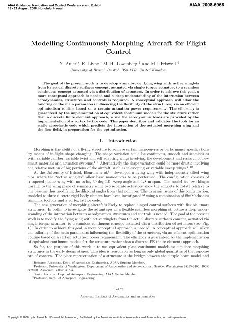
<strong>Modelling</strong> <strong>Continuously</strong> <strong>Morphing</strong> <strong>Aircraft</strong> <strong>for</strong> Flight<br />
Control<br />
N. Ameri ∗ , E. Livne † M. H. Lowenberg ‡ and M.I. <strong>Friswell</strong> §<br />
University of Bristol, Bristol, BS8 1TR, United Kingdom<br />
The goal of the present work is to develop a small-scale flying wing with active winglets<br />
from its actual discrete surfaces concept, actuated via single torque actuator, to a seamless<br />
continuous concept actuated via a distribution of actuators. In order to achieve this goal, a<br />
more conceptual approach is needed and a deep understanding of the interaction between<br />
aerodynamics, structures and controls is required. A conceptual approach will allow the<br />
tailoring of the main parameters influencing the flexibility of the structures, via an efficient<br />
optimisation routine based on a certain actuation power requirement. The efficiency is<br />
guaranteed by the implementation of equivalent continuum models <strong>for</strong> the structure rather<br />
than a discrete finite element approach, while the aerodynamic loads are provided by the<br />
implementation of a vortex lattice code. The paper describes and validates the tools <strong>for</strong> an<br />
static aeroelastic code which predicts the interaction of the actuated morphing wing and<br />
the flow field, in preparation <strong>for</strong> the optimisation.<br />
I. Introduction<br />
<strong>Morphing</strong> is the ability of a flying structure to achieve certain manoeuvres or per<strong>for</strong>mance specifications<br />
by means of in-flight shape changing. The shape variation could be continuous, smooth and seamless as<br />
with variable camber, variable twist and self adapting wings involving the development and research of new<br />
smart materials and actuation systems. 1–6 Alternatively the shape variation could be more drastic involving<br />
the relative motion of big portions of the aircraft, such as telescoping or variable sweep wings. 7–10<br />
At the University of Bristol, Bourdin et al. 11 developed a flying wing with independently tilted wing<br />
tips, where the “active winglets” allow basic manoeuvres to be per<strong>for</strong>med. The configuration consists of<br />
a tapered-planar wing with no twist, 30 deg LE sweep angle and 1.8 m span. The model has two hinges<br />
parallel to the wing plane of symmetry while two separate actuators allow the winglets to rotate relative to<br />
the baseline thus modifying the dihedral angles from that point on. The dynamic issues of this configuration,<br />
modeled as three discrete rigid-body element have been investigated 12 using a combination of SimMechanics<br />
Simulink toolbox and a vortex lattice code.<br />
The new generation of morphing aircraft is likely to replace hinged control surfaces with flexible smart<br />
structures. In order to investigate the advantages of a flexible seamless morphing structure a deep understanding<br />
of the interaction between aerodynamics, structures and controls is needed. The goal of the present<br />
work is to modify the flying wing with active winglets from the actual discrete surfaces concept, actuated via<br />
single torque actuator, to a seamless continuous concept actuated via a distribution of actuators (see Fig.<br />
1). In order to achieve this goal, a more conceptual approach is needed. A conceptual approach will allow<br />
the tailoring of the main parameters influencing the flexibility of the structures, via an efficient optimisation<br />
routine based on a certain actuation power requirement. The efficiency is guaranteed by the implementation<br />
of equivalent continuum models <strong>for</strong> the structure rather than a discrete FE (finite element) approach.<br />
So far, the purpose of this work is to use equivalent plate continuum models to simulate morphing<br />
structures in the early design stages. This idea is reasonable as long as only global quantities of the response<br />
are of concern. The plate representation of a structure is the bridge between the simple beam model and<br />
∗ Research Assistant, Dept. of Aerospace Engineering, AIAA Student Member.<br />
† Professor, University of Washington, Department of Aeronautics and Astronautics , Seattle, Washington 98195-2400, BOX<br />
352400. Associate Fellow AIAA.<br />
‡ Senior Lecturer, Dept. of Aerospace Engineering, AIAA Senior Member.<br />
§ Professor, Dept. of Aerospace Engineering.<br />
1 of 23<br />
American Institute of Aeronautics and Astronautics<br />
Copyright © 2008 by N. Ameri, M. I <strong>Friswell</strong>, M. Lowenberg. Published by the American Institute of Aeronautics and Astronautics, Inc., with permission.
Figure 1: Discrete and continuous morphing concept.<br />
the complex and accurate FE. Lovejoy and Kapania 13,14 listed more than 300 references concerning thin,<br />
thick, laminated or composite plates, whose geometry can be trapezoidal, and the lamina can be isotropic,<br />
orthotropic, or anisotropic in nature. Existing solutions <strong>for</strong> plates are classified according to the de<strong>for</strong>mation<br />
theory used, namely: the Classical Plate Theory (CPT), the First-order Shear De<strong>for</strong>mation Theory (FSDT),<br />
or the Higher-order Shear De<strong>for</strong>mation Theory (HSDT).<br />
The CPT is based on the Kirchhoff-Love hypothesis which states that a straight line normal to the<br />
plate middle surface remains straight and normal during the de<strong>for</strong>mation process. According to Reddy and<br />
Dawe 15,16 the CPT approach works well when through-thickness shear de<strong>for</strong>mations are negligible, that is<br />
true <strong>for</strong> thin isotropic plates. The FSDT, based on the Reissner-Mindlin model, 17,18 relaxes the constraint<br />
that a normal to the mid-surface stays normal to the mid-surface after de<strong>for</strong>mation, and a uni<strong>for</strong>m transverse<br />
shear strain is allowed. The FSDT, because of its simplicity, has a low computation requirement. On the<br />
other hand, the HSDT theory is based on a more accurate representation of the local distribution of the<br />
transverse shear. 19<br />
Structures using CPT, FSDT or HSDT can be modelled using finite element, Galerkin, and Rayleigh-<br />
Ritz approaches 13,14 but the the Rayleigh-Ritz method is more suited to conceptual design because of its<br />
computational efficiency. Giles 20,21 developed a Ritz method, which considers an aircraft wing as being<br />
<strong>for</strong>med by a series of equivalent trapezoidal segments, and represents the true internal wing box structure<br />
such as skin, caps, ribs and spars in the polynomial power <strong>for</strong>m. In Giles 20 the CPT was used and a symmetric<br />
airfoil section was assumed, but these shortcoming were removed subsequently. 21 Tizzi 22 presented a method<br />
to represent several trapezoidal segments in different planes, but the internal parts of wing box structures<br />
were not considered. Livne 23 <strong>for</strong>mulated the FSDT to model solid plates as well as typical wing box structures<br />
made of cover skins and an array of spars and ribs based on simple-polynomial trial functions, which are<br />
known to be prone to numerical ill-conditioning problems. Livne and Navarro 24 then further developed the<br />
method to deal with nonlinear problems of wing box structures. Kapania et al. 25–29 used the Rayleigh-Ritz<br />
method with Chebyshev polynomials as the trial functions and applied Lagrange’s equation to obtain the<br />
stiffness and mass matrices, although in all of these works only uni<strong>for</strong>m plates were considered. Subsequently,<br />
Kapania and Liu 30 extended the previous work using Legendre polynomials as the trial functions. The wing<br />
was composed of skins, spars and ribs and the Reissner-Mindlin displacement model was used. Finally Gern<br />
and Inman 31 investigated the roll per<strong>for</strong>mance and actuation power requirements of a generic smart wing<br />
plan<strong>for</strong>m and the results were compared with those of a conventional wing with trailing-edge flaps. The<br />
structure was described by an equivalent plate model assuming FSDT theory and Legendre polynomials as<br />
trial functions. The wing was divided into an inner and outer trapezoid, both comprising of ribs, spar, caps<br />
and skin, while <strong>for</strong> the aerodynamics a linearised compressible vortex lattice method was implemented. The<br />
overall model allowed static aeroelastic response analysis due to a fixed distributed actuation scheme. So<br />
far, no assessment has been made concerning the optimisation of the actuator distribution scheme in order<br />
to minimise actuation energy.<br />
Thus an equivalent plate model approach has been chosen <strong>for</strong> the present work instead of the widely used<br />
equivalent beam model which is not suitable <strong>for</strong> low aspect ratio wings made of composite materials. 32,33 The<br />
wing geometry is defined by a small number of sizing and shape design variables. Specifically the skin depth<br />
2 of 23<br />
American Institute of Aeronautics and Astronautics
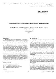
Figure 2: Generic trapezoidal wing (left) and wing box (right) schemes<br />
and thickness, spar caps, ribs and spar thicknesses are all defined through polynomials with respect to the<br />
coordinates of a reference plane where the wing trapezoid is defined. Similarly displacements can be defined<br />
by polynomials whose coefficients represent the time-dependent generalised coordinates. Minimisation of<br />
the total energy will lead to the Lagrange equations and the mass and stiffness matrices can be evaluated<br />
once by analytical integration. Consequently, these analytical espressions and the reduced size of the model<br />
guarantees that model initialisation and solution time <strong>for</strong> static and dynamic analyses are shorter than a<br />
detailed finite element model. Another advantage is that because the displacement functions are continuous<br />
over the plan<strong>for</strong>m, loads at the aerodynamic grid points can be transferred to the structure without the need<br />
<strong>for</strong> interpolation.<br />
For aeroelastic purposes a subsonic quasi-static 3D vortex lattice method is considered which is best<br />
suited <strong>for</strong> static aeroelastic analysis. Only a spanwise discretisation is taken into account so that the wing<br />
is divided into strips and <strong>for</strong> each strip induced drag, side <strong>for</strong>ce and lift can be evaluated. Because of the<br />
nature of the structural model no interpolation is needed in order to transfer the aerodynamic loads of each<br />
strip to the structural points. It has to be noted that with this approach the generalised aerodynamic <strong>for</strong>ces<br />
(GAF) are non-linear with respect to the generalised coordinates and an iterative method is needed in order<br />
to find the solution <strong>for</strong> each configuration.<br />
The paper is organised as follows: Section II firstly provides a description of theoretical aspects of the<br />
equivalent plate modelling and secondly the static and dynamic properties of a wing box are used to validate<br />
the modelling. Section III provides a description of the actuator modelling, and the implementation of<br />
devices based on piezo-thermo strain actuation, as well as external <strong>for</strong>ces, is shown. Section IV provides a<br />
theoretical overview of the vortex lattice code and again, results validating the model are shown. Finally<br />
in section V the aeroelasto-static system together with the results from a preliminary parametric study, are<br />
discussed. Conclusions are presented in Section VI.<br />
II.A.<br />
Geometry Definition<br />
II. Structural Modeling<br />
The geometry of the wing is shown in Fig. 2. It represents a generic trapezoidal wing shape defined over a<br />
global left-handed coordinate system x, y and z and comprising of spars, ribs and caps. The wing can be<br />
defined over the following bounded set<br />
x : {x 1 + y tan (Λ LE ) < x < x 1 + y tan(Λ LE ) + c(y)}<br />
y : {y 1 < y < y 2 }<br />
(1)<br />
where Λ LE is the leading edge sweep angle and c(y) is the local chord. A depth distribution, which is the<br />
height of each composite skin layer <strong>for</strong>ming the wing shape with respect to a reference plane z = 0, can be<br />
defined over the bounded region of the wing. The i-th layer height z ski can be described by a polynomial<br />
3 of 23<br />
American Institute of Aeronautics and Astronautics
series in the x and y global coordinates as follows<br />
∑N k<br />
z ski (x, y) = H ski<br />
k<br />
x m k<br />
y n k<br />
(2)<br />
k=1<br />
where the H ski<br />
k<br />
coefficients can be used as design variables. Under the hypothesis of a small thickness-todepth<br />
ratio only two sets of depth can be taken into account, namely the upper and lower surface, z up and<br />
z lo . In a similar manner, a distribution of the i-th composite layer thickness can be defined over the wing<br />
plat<strong>for</strong>m<br />
N<br />
∑ j<br />
t ski (x, y) = T ski<br />
j<br />
x mj y nj (3)<br />
Each spar can be identified by a spar line having the general expression<br />
j=1<br />
x spj (y) = a 1 y + a 2 (4)<br />
This linear equation locates the η axis of a local coordinates system (ξ, η, z) which is rotated with respect to<br />
the global system by an angle Λ spj . The thickness distribution and cap area of the spars can be expressed as<br />
simple polynomials in y, t spj (y) and A spj (y) respectively. Each rib is modeled as parallel to the longitudinal<br />
axis, and thus is identified simply by the line y = y rb k<br />
, with thickness distribution t rb k<br />
(x) and spar cap area<br />
A rb k<br />
(x).<br />
II.B. Material Properties<br />
Each skin layer has its own fibre direction in the x, y plane and the constitutive equations reflect a plane<br />
strain behavior (ε zz = 0) a σ ski = Q ski ǫ ski (5)<br />
where σ ski = [σ xx , σ yy , σ xy ] T and ǫ ski = [ε xx , ε yy , γ xy ] T are the stress and strain vectors respectively. Q ski<br />
is the constitutive matrix of the i-th layer.<br />
The constitutive behaviour of each spar is defined in the local ξ, η, z coordinate system so that<br />
˜σ spj = ˜Q spj˜ǫ spj (6)<br />
where ˜σ spj = [σ ηη , σ xz ] T and ˜ǫ spj = [ε ηη , γ ηz ] T . This means that the spars sustain only axial stress and the<br />
transverse shear. The spar strain vector in global coordinates ǫ spj = [ε xx , ε yy , γ xy , γ xz , γ yz ] T is related to<br />
the strain in local coordinates by means of the following relation 36<br />
˜ǫ spj = T ǫ spj (7)<br />
where T is the global-to-local rotation matrix <strong>for</strong> the spar strain vector defined as<br />
[<br />
]<br />
s<br />
T =<br />
2 (Λ spj ) c 2 (Λ spj ) s(Λ spj )c(Λ spj ) 0 0<br />
0 0 0 s(Λ spj ) c(Λ spj )<br />
Spar caps sustain only axial stress, and thus the constitutive equation is simply<br />
A rotation vector gives the global to local trans<strong>for</strong>mation<br />
σ ηη = E ε ηη (9)<br />
ε ηη = t T ǫ spcr (10)<br />
where ǫ spcr = [ε xx , ε yy , γ xy ] T is the spar cap strain vector in global coordinates and the rotation matrix is<br />
given by<br />
[<br />
] T<br />
t = s 2 (Λ spj ) c 2 (Λ spj ) s(Λ spj )c(Λ spj )<br />
(11)<br />
Similar relations can be obtained easily <strong>for</strong> the ribs and the rib caps. They behave in a similar way to<br />
the spars and spar caps previously described, but the local η axes is rotated by an angle Λ rb k<br />
= 90 ◦ and<br />
coincides with the x axis.<br />
a Unless stated otherwise, in this paper vectors will be defined using a bold lower case notation while a bold upper case<br />
notation will be used <strong>for</strong> matrices.<br />
(8)<br />
4 of 23<br />
American Institute of Aeronautics and Astronautics
II.C.<br />
First-Order Shear De<strong>for</strong>mation Kinematic Assumption<br />
The first-order shear de<strong>for</strong>mation plate theory (FSDT) is based on the Reissner-Mindlin 17,18 assumption<br />
where the u, v and w displacements of the wing are approximated as<br />
u(x, y, z, t) = u 0 (x, y, t) + zψ x (x, y, t)<br />
v(x, y, z, t) = v 0 (x, y, t) + zψ y (x, y, t) (12)<br />
w(x, y, z, t) = w 0 (x, y, t)<br />
where u 0 , v 0 and w 0 are the displacements at the reference plane (z = 0), and ψ x and ψ y are the unknown<br />
functions giving contributions to the transverse shear de<strong>for</strong>mations in the x-z and y-z direction respectively.<br />
The classical plate theory (CPT), where shear effects are neglected, can be obtained by simply substituting<br />
in Eq. (12) the following expressions <strong>for</strong> the rotations<br />
ψ x = −w ,x<br />
ψ y = −w ,y<br />
(13)<br />
Under the hypothesis of small surface curvatures, the skins can be modeled as a thin plane stress panel, and<br />
the strain field is given by<br />
ε xx = u ,x<br />
ε yy = v ,y (14)<br />
γ xy = u ,y + v ,x<br />
while the transverse shear field, captured by spars and ribs, are<br />
γ xz = u ,z + w ,x<br />
γ yz = v ,z + w ,y<br />
(15)<br />
Substituting Eqs. (12) into Eqs. (15) it is possible to show that ψ x and ψ y are the actual rotations of the<br />
sections about the y and x axes respectively<br />
ψ x = γ xz − w 0,x<br />
ψ y = γ yz − w 0,y<br />
(16)<br />
If a classical plate theory is assumed only the terms w 0,x and w 0,y would be non-zero and the sections normal<br />
to the middle plane would stay normal after the rotation.<br />
II.D.<br />
Mass and Stiffness Matrices<br />
The equivalent plate theory is based on the assumption that all of the de<strong>for</strong>mation field is approximated by<br />
a series of Ritz polynomials. Thus the unknowns in Eqs. (12) can be expressed as<br />
u 0 (x, y, t)<br />
v 0 (x, y, t)<br />
= a 1 (x, y) T q 1 (t)<br />
= a 2 (x, y) T q 2 (t)<br />
ψ x (x, y, t) = a 3 (x, y) T q 3 (t) (17)<br />
ψ y (x, y, t)<br />
w 0 (x, y, t)<br />
= a 4 (x, y) T q 4 (t)<br />
= a 5 (x, y) T q 5 (t)<br />
where a i = [. . . , x np y mp , . . .] T are vectors containing the polynomial terms or shape functions, which may be<br />
of different lengths. The q i are vectors of the time-dependent generalised coordinates. Substituting Eqs. (17)<br />
into Eqs. (12) and defining the displacement vector u = [u, v, w] T and the vector of generalised coordinates<br />
q = [q T 1 ,qT 2 ,qT 3 ,qT 4 ,qT 5 ]T , leads to<br />
u = S q (18)<br />
5 of 23<br />
American Institute of Aeronautics and Astronautics
where S = S(x, y, z) is the matrix relating the generalised coordinates to the physical displacements. Substituting<br />
Eqs. (17) into Eqs. (14) and Eqs. (15) leads to<br />
ǫ ski = E q (19)<br />
ǫ spj = W q (20)<br />
where E = E(x, y, z) and W = W(x, y, z) are matrices providing the de<strong>for</strong>mation field <strong>for</strong> the skin layers<br />
and <strong>for</strong> the spars respectively.<br />
Finally, the mass and stiffness matrices <strong>for</strong> each element of the wing are obtained using an energy<br />
approach. Specifically, kinetic (T ) and elastic potential (E) contributions to the total energy of the wing<br />
will be defined <strong>for</strong> the skin, spar and spar caps (the procedure is identical <strong>for</strong> ribs and rib caps) and the<br />
application of the Lagrange equations<br />
d<br />
dt<br />
( ∂T<br />
∂ ˙q n<br />
)<br />
− ∂T<br />
∂q n<br />
+ ∂E<br />
∂q n<br />
= 0 (n = 1, 2, . . ., N q ) (21)<br />
minimises the total energy with respect to the generalised coordinates, and will give the mass and stiffness<br />
matrices. In practice, this procedure requires the computation of integrals over the geometric domain but,<br />
because of the nature of the shape functions and the definition of depths, thicknesses and areas given in Sec.<br />
II.A, which are all polynomials in x and y, the integrals may be calculated in closed <strong>for</strong>m, and no numerical<br />
evaluation is needed.<br />
II.D.1. Skin<br />
The contribution to the kinetic energy of an infinitesimal skin element of volume t ski (x, y)dxdy and of ̺<br />
density, is given by<br />
dT ski = 1 2 ̺ tski (x, y) ˙u T ˙u dx dy (22)<br />
Substituting Eq. (18) and integrating over the wing domain defined in Eq. (1), gives the total kinetic energy<br />
as<br />
T ski = 1 (∫∫<br />
)<br />
2 ˙qT ̺ t ski (x, y) S(x, y, z ski ) T S(x, y, z ski ) dx dy ˙q<br />
= 1 2 ˙qT M ski ˙q (23)<br />
Similarly the potential energy of the infinitesimal skin element is<br />
dE ski = 1 2 tski (x, y) ǫ skiT σ ski dx dy (24)<br />
Substituting Eqs. (5) and (19) and integrating over the wing domain, gives the total potential energy as<br />
E ski = 1 (∫∫<br />
)<br />
2 qT t ski (x, y) E(x, y, z ski ) T Q ski E(x, y, z ski ) dx dy q<br />
= 1 2 qT K ski q (25)<br />
II.D.2. Spar<br />
The contribution to the kinetic energy of an infinitesimal spar element of volume t spj (η)dηdz and of ̺ density,<br />
is given by<br />
dT spj = 1 2 ̺ tspj (η) ˙u T ˙u dη dz (26)<br />
Again substituting Eq. (18) and considering the global to local coordinate system relation<br />
dη = dy/cos(Λ spj ) (27)<br />
6 of 23<br />
American Institute of Aeronautics and Astronautics
the double integration over the wing length and between the lower an upper limit of the spar, leads to the<br />
following expression <strong>for</strong> the mass matrix as<br />
M spj =<br />
̺<br />
cos(Λ spj )<br />
∫ z up (x sp j ,y) ∫ y2<br />
z lo (x sp j ,y)<br />
y 1<br />
t spj (y) S(x spj , y, z) T S(x spj , y, z) dy dz (28)<br />
where x spj = x spj (y) is the spar line as defined in Eq. (4). The potential energy of the infinitesimal spar<br />
element is defined as<br />
dU spj = 1 (η) ˜ǫ<br />
2 tspj spj T ˜σ spj dη dz (29)<br />
Eqs. (6), (7), (20) and (27) give the expression <strong>for</strong> the spar stiffness matrix<br />
K spj =<br />
1<br />
cos(Λ spj )<br />
II.D.3. Spar Caps<br />
∫ z up (x sp j ,y) ∫ y2<br />
z lo (x sp j,y)<br />
y 1<br />
t spj (y) E(x spj , y, z) T T(Λ spj ) T ˜Q spj T(Λ spj ) E(x spj , y, z) dy dz (30)<br />
The volume of an infinitesimal spar cap element, belonging to the j-th spar, is A spcr (y)dηdx. Thus, following<br />
the procedure adopted in the previous section, expressions <strong>for</strong> the mass and stiffness matrices <strong>for</strong> the spar<br />
caps are<br />
K spcr =<br />
̺<br />
M spcr =<br />
cos(Λ spj )<br />
E<br />
cos(Λ spj )<br />
∫ y2<br />
∫ y2<br />
y 1<br />
A spcr (y) S(x spj , y, z ∗ ) T S(x spj , y, z ∗ ) dy (31)<br />
y 1<br />
A spcr (y) W(x spj , y, z ∗ ) T t t T W(x spj , y, z ∗ ) dy (32)<br />
where z ∗ = z up/lo (x spj , y) is the height at which the spar cap is defined.<br />
Finally mass and stiffness matrices of the whole structure are given by summing the contributions of all<br />
the elements of the wing.<br />
M = ∑ M ski + ∑ M spj + ∑ M spcr + ∑ M rb k<br />
+ ∑ M rbcs (33)<br />
K = ∑ K ski + ∑ K spj + ∑ K spcr + ∑ K rb k<br />
+ ∑ K rbcs (34)<br />
II.E. Validation<br />
The theory has been implemented in two stages: Firstly Maple was used to generate, according to the<br />
theory in the previous sections, expressions <strong>for</strong> the mass and the stiffness matrices of each element of the<br />
wing; these matrices are parametric with respect to a certain number of selected design variables. Secondly<br />
these expressions have been exported to Matlab and functions have been generated <strong>for</strong> this purpose. The<br />
process has to be repeated when a different set of design parameters (i.e. a different set of shape functions<br />
<strong>for</strong> the displacements) is required, but if this set is fixed, only Matlab is involved to the simulations.<br />
A test case has been selected in order to validate the structural model consisting of a cantilevered wing box<br />
made of aluminum. In order to represent the wing box behavior, the following complete set of polynomials<br />
were chosen to approximate the displacements given by Eqs. (17)<br />
a 1 (x, y) =<br />
a 2 (x, y) =<br />
[1, x, y, x 2 , xy, y 2 , x 3 , x 2 y, xy 2 , y 3 ] T<br />
[1, x, y, x 2 , xy, y 2 , x 3 , x 2 y, xy 2 , y 3 ] T<br />
a 3 (x, y) = [1, x, y, x 2 , xy, y 2 , x 3 , x 2 y, xy 2 , y 3 , x 4 , x 3 y, x 2 y 2 , xy 3 , y 4 ] T (35)<br />
a 4 (x, y) = [1, x, y, x 2 , xy, y 2 , x 3 , x 2 y, xy 2 , y 3 ] T<br />
a 5 (x, y) = [1, x, y, x 2 , xy, y 2 , x 3 , x 2 y, xy 2 , y 3 , x 4 , x 3 y, x 2 y 2 , xy 3 , y 4 , x 5 , x 4 y, x 3 y 2 , x 2 y 3 , xy 4 , y 5 ] T<br />
while the boundary condition at the wing root is satisfied by placing a set of very stiff rotational and linear<br />
springs which restricts the rotations and displacements of the section. A sensitivity analysis is needed to<br />
select these values: too soft springs would lead to a misrepresentation of the cantilever condition, while too<br />
stiff springs would cause ill-conditioning. The use of springs to en<strong>for</strong>ce the boundary condition is necessary<br />
7 of 23<br />
American Institute of Aeronautics and Astronautics
ecause the chosen set of polynomials allows the rigid modes of the plate. Moreover, assuming a set of<br />
complete polynomials will allow (see Sec. II.F) the easy implementation of multiple plate capability of plates<br />
with arbitrary orientation in space, as <strong>for</strong> each body in the system is represented by the same set of shape<br />
functions.<br />
The choice of shape functions previously made yields a total number of 66 dof. If the transverse shears are<br />
neglected and a CPT is assumed then the number of dof decreases to 41. The main geometrical parameters<br />
of the wing box are reported in Tab. 1; the wing box has rectangular section (see Fig. 3) with structural<br />
chord b which is half of the aerodynamic chord c while the depth is set to h = .1c. The wing has a front<br />
and a rear spar and a web of three ribs equally spaced along the wing of length L. Each spar and rib carries<br />
two caps having area A. Skin, spars and ribs are assumed to have the same thickness t which is constant<br />
all over the wing. Two cases of leading edge sweep angle are considered <strong>for</strong> the current validation, namely<br />
E 70 GPa<br />
ν 0.35 -<br />
ρ 2700 Kg/m 3<br />
L 0.8 m<br />
c 0.3 m<br />
t 4 10 −3 m<br />
A cap 10 −4 m 2<br />
N spar 2 -<br />
N rib 3 -<br />
Figure 3: Wing-box scheme.<br />
Table 1: Material and geometrical properties of the<br />
wing box.<br />
Λ LE = 0 ◦ and Λ LE = 30 ◦ . Finally, expressions <strong>for</strong> the mass and the stiffness matrices can determined as<br />
M = M(ρ; b, h, L, Λ LE , t, A cap , N spar , N rib ) (36)<br />
K = K(E, ν; b, h, L, Λ LE , t, A cap , N spar , N rib ) (37)<br />
In order to validate the structural tool, an accurate model of the wing box has been built and analysed using<br />
NASTRAN. Skin, ribs and spars are modelled by CQUAD4 elements while the caps are modelled by CROD<br />
elements, leading to a total number of 6600 dof.<br />
II.E.1. Static validation<br />
In terms of static analysis only the stiffness matrix is involved, and two load cases are considered<br />
1. a concentrated vertical <strong>for</strong>ce F z = 1 N<br />
2. a concentrated torque M y = 1 Nm about the y axis<br />
both applied at the middle chord of the tip section. It has to be noted that a single concentrated load<br />
represents the most critical situation <strong>for</strong> the equivalent plate model which is best suited <strong>for</strong> distributed<br />
loads. the reason is because the method tends to smear local effects over the wing area, and so localized<br />
load effects are averaged over the whole domain. These two cases have been selected in order to investigate<br />
the limits of the method.<br />
The results <strong>for</strong> the first case are shown in Fig. 4. Specifically, the vertical displacements w of the<br />
middle chord of the tip section are shown, both <strong>for</strong> an unswept wing and a 30 ◦ swept wing. For each<br />
case displacements obtained from the CPT, FSDP and NASTRAN are compared. The rotations of the tip<br />
section, the consequence of an applied unitary torque, are shown in Fig. 5. Finally, the relative errors with<br />
respect to the NASTRAN results are shown in Tab. 2. The FSDP shows the maximum relative error of<br />
8.4% <strong>for</strong> the tip vertical displacement, corresponding to the 30 ◦ swept wing with applied vertical <strong>for</strong>ce at<br />
the wing tip. In all the other cases the error is under 4%. The CPT exibits a maximum error of 26.5% <strong>for</strong><br />
the rotation corresponding to the 30 ◦ swept wing with applied torque at the wing tip. Note that the FSDP<br />
theory gives results which are more accurate than the CPT. Moreover, the CPT overestimates the stiffness<br />
matrix leading to a wing whose overall behavior is stiffer than the FE model.<br />
8 of 23<br />
American Institute of Aeronautics and Astronautics
Vertical displacement [m] (ΛLE = 0 ◦ )<br />
7 x 10⁻⁶<br />
6<br />
5<br />
4<br />
3<br />
2<br />
1<br />
0<br />
CPT<br />
FSDPT<br />
Nastran<br />
1 2 3<br />
Vertical displacement [m] (ΛLE = 30 ◦ )<br />
1.2 x 10⁻⁵<br />
1<br />
0.8<br />
0.6<br />
0.4<br />
0.2<br />
0<br />
1 2 3<br />
CPT<br />
FSDPT<br />
Nastran<br />
Figure 4: Vertical displacements at the middle chord of the tip section <strong>for</strong> F z = 1 N and sweep angles<br />
Λ LE = 0 ◦ (left) and Λ LE = 30 ◦ (right).<br />
9 x 10⁻⁶<br />
1.2 x 10⁻⁵<br />
Rotation [rad] (ΛLE = 0 ◦ )<br />
8<br />
7<br />
6<br />
5<br />
4<br />
3<br />
2<br />
1<br />
0<br />
1 2 3<br />
CPT<br />
FSDPT<br />
Nastran<br />
Rotation [rad] (ΛLE = 30 ◦ )<br />
1<br />
0.8<br />
0.6<br />
0.4<br />
0.2<br />
0<br />
1 2 3<br />
CPT<br />
FSDPT<br />
Nastran<br />
Figure 5: Rotations of the tip section <strong>for</strong> M y = 1 Nm and sweep angles Λ LE = 0 ◦ (left) and Λ LE = 30 ◦<br />
(right).<br />
II.E.2. Dynamic validation<br />
The capability of the equivalent plate modelling <strong>for</strong> the prediction of natural frequencies and mode shapes<br />
<strong>for</strong> the same wing box, is discussed in this section. The present analysis involves only the FSDP theory which<br />
was shown, by the analysis in the previous section, to be more accurate than the CPT. Two configurations<br />
are considered, namely the unswept wing box and the 30 ◦ swept-back wing box. In order to evaluate the<br />
eigensystem of the wing box, both the mass and stiffness matrices have to be calculated via the equivalent<br />
plate theory. The procedure produces matrices with a block-diagonal structure.<br />
Eigenvalues and eigenvectors of the equivalent plate structural system are evaluated via the Matlab<br />
“eig” function, and compared with those obtained from the FE code. The first five natural frequencies,<br />
corresponding to the two configurations considered, are shown in Tab. 3 with the associated relative errors.<br />
These results show that the NASTRAN and the FSDPT frequencies are in good agreement, <strong>for</strong> both the<br />
unswept and back-swept configurations, <strong>for</strong> the first three modes, namely the first bending, the first in plane<br />
bending and the second bending modal shapes: in all these cases the maximum error is about 4.18%. The<br />
correlation is not possible <strong>for</strong> the modes above the fourth mode shape and this is due to the polynomial<br />
order chosen <strong>for</strong> the present analysis; higher modes can be estimated using higher polynomial order even<br />
though this would lead to an increase in the number of dof and the overall size of the system. In Fig. 6 the<br />
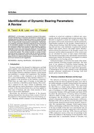
first four mode shapes can be seen and compared directly with those from NASTRAN.<br />
II.F.<br />
Multiple Plate Capability<br />
If the system comprises of more than one plate, each of them with arbitrary orientation in space, a global<br />
coordinate system has to be set up. A local coordinate system, fixed with respect to the unde<strong>for</strong>med reference<br />
state, can be defined <strong>for</strong> each plate. Thus if the same set of polynomials is used <strong>for</strong> each plate, the global<br />
9 of 23<br />
American Institute of Aeronautics and Astronautics
Figure 6: Comparison between FSDPT modal shapes (left) and NASTRAN modal shapes (right).<br />
10 of 23<br />
American Institute of Aeronautics and Astronautics
% Λ LE = 0 ◦ Λ LE = 30 ◦<br />
ε CPT<br />
w 8.19 8.6<br />
ε FSDP<br />
w 0.85 8.4<br />
ε CPT<br />
θ<br />
23.1 26.5<br />
ε FSDP<br />
θ 3.9 3.94<br />
Table 2: CPT and FSDP errors relative to NASTRAN results <strong>for</strong> the wing box example.<br />
Λ LE = 0 ◦ Λ LE = 30 ◦<br />
Mode # f NAS [Hz] f FSDPT [Hz] ε [%] f NAS [Hz] f FSDPT [Hz] ε [%]<br />
1 57.87 56.84 1.7 44.19 45.17 -2.2<br />
2 219.95 215.58 1.2 151.17 154.27 -2.05<br />
3 315.32 323.22 -2.5 247.30 254.56 -2.9<br />
4 356.42 370.37 -3.9 342.75 357.1 -4.18<br />
5 705.58 1089 -54.4 596.80 688.07 -15.3<br />
Table 3: Natural frequencies <strong>for</strong> the wing box example.<br />
number of degrees of freedom will be N P ×N q where N P is number of plates and N q is the number of degrees<br />
of freedom of each plate. Finally each plate will add to the system a contribution to the kinetic and potential<br />
energy that is evaluated with respect to the local coordinate system and thus the <strong>for</strong>mulation obtained in<br />
previous sections will be used <strong>for</strong> this purpose.<br />
In the current <strong>for</strong>mulation the displacement compatibility between contiguous plates is imposed by means<br />
of stiff springs. In contrast to Demasi, 34 where only longitudinal springs were placed throughout the thickness<br />
to impose the cantilever condition and the compatibility, both rotational and longitudinal springs will be<br />
used in this work. The displacement compatibility is imposed in global coordinates but expressed in local<br />
coordinates as follows: Consider the contiguous plates i and j and let R i and R j be respectively the global<br />
to local tras<strong>for</strong>mation matrix of each plate. In order to impose the displacement compatibility of the point<br />
A i belonging to body i and the point A j belonging to body j the following expression leads to the potential<br />
energy of the springs linking A i and A j<br />
⎡<br />
E = 1 2 (ūi A i<br />
− ū j A j<br />
) T ⎢<br />
⎣<br />
⎤<br />
k x 0 0 0 0<br />
0 k y 0 0 0<br />
0 0 k z 0 0<br />
⎥<br />
0 0 0 k rx 0 ⎦<br />
0 0 0 0 k ry<br />
(ū i A i<br />
− ū j A j<br />
) (38)<br />
where ū collects the elastic displacements and the rotations of a point of the structure in global coordinates.<br />
Thus the global displacement vector can be expressed first in terms of the local displacement ū, via a<br />
geometrical rotation matrix, and, consequently, in terms of the Lagrangian coordinates via the matrix of<br />
shape functions S.<br />
ū = R u = R S q (39)<br />
Substituting Eq. (39) in to Eq. (38) leads to the following expression <strong>for</strong> the potential energy<br />
E = 1 2 (qT i K s ii q i + q T j K s jj q j + q T i K s ij q j + q T j K s ji q i ) (40)<br />
11 of 23<br />
American Institute of Aeronautics and Astronautics
where the generic contribution to the stiffness matrix is defined as<br />
⎡<br />
⎤<br />
k x 0 0 0 0<br />
0 k y 0 0 0<br />
K s lp = S T A l<br />
R lT 0 0 k<br />
⎢<br />
z 0 0<br />
R p S Ap<br />
⎥<br />
⎣ 0 0 0 k rx 0 ⎦<br />
0 0 0 0 k ry<br />
<strong>for</strong> l = i, j; p = i, j (41)<br />
Hence, each set of springs introduces contributions to the stiffness matrix of each plate and a cross contribution<br />
between plates so that the global stiffness matrix can be assembled as follows<br />
⎡<br />
⎤<br />
. .. K ii + K s ii K s ij<br />
K =<br />
⎢<br />
⎣<br />
K s ji K jj + K s (42)<br />
⎥<br />
jj ⎦<br />
. ..<br />
and the vector of generalised coordinates of the assembed system is<br />
q = [ . . .,q T i ,qT j , . . .] T<br />
(43)<br />
The mass matrix can be assembled in a similar way but no cross contributions will appear.<br />
III. Piezo and Thermo Actuator <strong>Modelling</strong> <strong>for</strong> Equivalent Plate<br />
A patch of piezo or thermo actuator undergoes a strain variation when an electrical field or a thermal<br />
variation respectively, is imposed through the thickness. Assuming that the patches are thin enough to be<br />
modelled as plates and assuming a plane-strain behavior, the previous relations can be expressed analytically<br />
by the following<br />
⎡ ⎡ ⎤<br />
⎤<br />
ε 11<br />
⎢ ⎥ ⎢<br />
˜ǫ ∆T = ⎣ ε 22 ⎦ = ⎣<br />
γ 12<br />
⎡ ⎤ ⎡<br />
ε 11<br />
⎢ ⎥ ⎢<br />
˜ǫ V = ⎣ ε 22 ⎦ = ⎣<br />
γ 12<br />
α 1<br />
α 2<br />
0<br />
d 13<br />
d 23<br />
0<br />
⎥<br />
⎦∆T (44)<br />
where ˜ǫ ∆T and ˜ǫ V are the strains defined in the principal material coordinates of each patch, α 1 and α 2<br />
[ ◦ C −1 ] are the thermal expansion coefficients in the 1 and 2 directions respectively, d 13 and d 23 [m/V ] are<br />
the piezoelectric constants; ∆T is the temperature variation input with respect to a reference temperature<br />
while the ratio V/t, between the input voltage V and the distance between the electrodes t, represents the<br />
through-the-thickness electric field.<br />
The strain vectors in global coordinates ǫ ∆T and ǫ V , can be obtained applying the rotation matrix T<br />
which is a function of the angle θ that defines the orientation of the principal material coordinate system<br />
with respect to the global, and is defined as follows<br />
such that<br />
T(θ) =<br />
⎡<br />
⎢<br />
⎣<br />
⎤<br />
m 2 n 2 mn<br />
n 2 m 2 −mn<br />
−2mn 2mn m 2 − n 2<br />
⎤<br />
⎥<br />
⎦ V t<br />
(45)<br />
⎥<br />
⎦ m = cos(θ) n = sin(θ) (46)<br />
˜ǫ = T(θ) ǫ (47)<br />
Using this definition, the strain vectors in global coordinates can be obtained as<br />
ǫ ∆T = T(θ) −1 b ∆T ∆T<br />
ǫ V = T(θ) −1 V<br />
b V t<br />
(48)<br />
12 of 23<br />
American Institute of Aeronautics and Astronautics
where b ∆T = [α 1 , α 2 , 0] T and b V = [d 13 , d 23 , 0] T .<br />
The strain due to the stress field ǫ S is obtained subtracting from the total strain field ǫ the contribution<br />
due to the thermal and the piezoelectric strains.<br />
ǫ S = ǫ − ǫ ∆T − ǫ V (49)<br />
Recalling Eq. (19), linking the total strain vector to the generalised coordinates vector <strong>for</strong> an infinitesimal<br />
skin element, and Eqs. (48), the previous equation becomes<br />
ǫ S = E q − T(θ) −1 b ∆T ∆T − T(θ) −1 b V<br />
V<br />
t<br />
(50)<br />
The constitutive relations that provide the stress vector σ = [σ xx , σ yy , σ xy ] T is given by<br />
σ = Q ǫ S (51)<br />
where Q is the constitutive matrix rotated in global coordinates. The equations describing the interaction<br />
between the smart patches and the structure will be obtained via a virtual work approach. The virtual work<br />
δW ε done by the elastic <strong>for</strong>ces on an infinitesimal element of piezo-thermo actuator of volume t dxdy can be<br />
defined as follow<br />
δW ε = δǫ T σ t dx dy<br />
(<br />
)}<br />
= δq<br />
{E T T Q E q − T(θ) −1 b ∆T ∆T − T(θ) −1 V<br />
b V<br />
t<br />
t dx dy (52)<br />
The inertial <strong>for</strong>ces f i acting on an infinitesimal element of mass ̺tdxdy can be defined using d’Alembert<br />
principle as<br />
f i<br />
= −̺ t ü dx dy<br />
= −S ¨q ̺ t dx dy (53)<br />
Thus, the virtual work δW i done by the inertial <strong>for</strong>ces becomes<br />
δW i = δu T f i<br />
= −δq T S T S ¨q ̺ t dx dy (54)<br />
In a similar way, the virtual work δW ext done by the external <strong>for</strong>ces f ext per unit area, can be defined as<br />
δW ext<br />
= δu T f ext dx dy<br />
= δq T S T f ext dx dy (55)<br />
The equilibrium condition states that the external and inertial virtual works must balance the internal<br />
work done by the stresses<br />
δW ext = δW i + δW ε (56)<br />
Substituting in the previous equation, Eqs. (52), (54) and (55), lead to<br />
{<br />
}<br />
δq T E T Q E q − E T Q T(θ) −1 b ∆T ∆T − E T Q T(θ) −1 V<br />
b V<br />
t<br />
which can be integrated over the area S A of the actuator patch, leading to<br />
t dx dy =<br />
= δq T { −̺ t S T S ¨q + S T f ext<br />
}<br />
dx dy (57)<br />
M A ¨q + K A q = e ext + e V V + e ∆T ∆T (58)<br />
13 of 23<br />
American Institute of Aeronautics and Astronautics
where<br />
M A =<br />
K A =<br />
e ext =<br />
e V =<br />
e ∆T =<br />
∫∫<br />
S T S ̺ t dx dy (59)<br />
S<br />
∫∫<br />
A E T Q E t dx dy (60)<br />
S<br />
∫∫<br />
A S T f ext dx dy (61)<br />
S<br />
(∫∫<br />
A )<br />
E T Q T(θ) −1 dx dy b V (62)<br />
S<br />
(∫∫<br />
A )<br />
E T Q T(θ) −1 t dx dy b ∆T (63)<br />
S A<br />
where M A and K A are the mass and stiffness contributions of the strain actuator to be added to the total<br />
mass and stiffness matrices of the structure, while e V and e ∆T are the generalized vectors providing to the<br />
structure the effect of an applied voltage and a temperature variation, respectively. If N A actuators are<br />
placed over the wing surface, the contribution of each actuator has to be included. If the patch dimensions<br />
are small compared to the whole skin area, then the previous equations can be discretized and evaluated<br />
with respect to the centre point coordinates of the patch, namely x A , y A and z A . For instance Eq. (59)<br />
becomes<br />
M A = S(x A , y A , z A ) T S(x A , y A , z A ) ̺ t a b (64)<br />
where a and b are the width and length of the patch, supposed to be rectangular.<br />
III.A.<br />
Validation via Thermal Analogy<br />
The strain actuation theory developed in the previous section will be validated taking into account only a<br />
static thermal load distribution and results from a finite element thermal analysis will be used <strong>for</strong> comparison.<br />
The validity of the method <strong>for</strong> the piezo patches can be easily extended using the thermal analogy. 35<br />
The wing box chosen as a test case is the same as in Sec. II.E <strong>for</strong> the 30 ◦ back-swept case. Indeed, the<br />
same NASTRAN finite element model is adopted.<br />
A distribution of thermal load is applied all over the upper skin (see Fig. 7). Specifically, the difference<br />
in temperature ∆T follows a quadratic law along the span, with maximum value at the mid-span, while no<br />
dependency is assumed along the chord direction, and thus<br />
[ ( y<br />
) ( ] y 2<br />
∆T(x, y) = 4∆T ∗ −<br />
(65)<br />
L L)<br />
where ∆T ∗ is the maximum value of the temperature field, occurring at y = L/2.<br />
In NASTRAN this has been done, within the static SOL 101 solver, via the TEMP card which allows an<br />
absolute temperature to be imposed at each nodes. However the reference temperature value, at which the<br />
coefficient of thermal expansion is evaluated (α 1 = α 2 = 23 × 10 −6 K −1 at 20 ◦ <strong>for</strong> Aluminium), has to be<br />
set in the MAT1 card. The equivalent plate thermal load model is obtained by discretisating the continuous<br />
distribution in Eq. (65), as described in III.<br />
Since the system is linear, results corresponding to a ∆T ∗ parameter equal to the unitary value are<br />
presented. In Fig. 8 the vertical displacements of the points belonging to the upper skin, both along<br />
the chord section at the half span and the section at the tip, are shown. Indeed, in Fig. 9 the vertical<br />
displacements of the points of the front and rear spar, belonging to the medium plane, are plotted. In the<br />
same figures, the displacements evaluated with the equivalent plate approach are compared with those from<br />
NASTRAN. The results are in good agreement, as the MAC (Modal Assurance Criterion) and the the MSF<br />
(Modal Scale Factor) between the two de<strong>for</strong>mation shapes are both equal to 0.97. Finally in Fig. 10, the<br />
von Mises stresses of points belonging to the upper skin above the elastic line, are plotted. Again the results<br />
are in good agreement and the maximum stress value is identified by the equivalent plate theory with an<br />
error of 0.8% relative to the NASTRAN prediction.<br />
14 of 23<br />
American Institute of Aeronautics and Astronautics
2 x 10⁻⁵<br />
Vertical displacement [m]<br />
0<br />
−2<br />
−4<br />
−6<br />
−8<br />
−10<br />
EP: half-span chord<br />
FE: half-span chord<br />
EP: tip chord<br />
FE: tip chord<br />
Figure 7: Thermal load distribution on the upper<br />
skin.<br />
−12<br />
0 0.1 0.2 0.3 0.4 0.5 0.6 0.7 0.8 0.9 1<br />
Non-dimentional chord<br />
Figure 8: Half span chord and tip chord displacements<br />
(∆T ∗ = 1).<br />
Vertical displacement [m]<br />
0<br />
−2<br />
−4<br />
−6<br />
−8<br />
−10<br />
2 x 10⁻⁵<br />
EP: leading edge<br />
FE: leading edge<br />
EP: trailing edge<br />
FE: trailing edge<br />
−12<br />
0 0.1 0.2 0.3 0.4 0.5 0.6 0.7 0.8 0.9 1<br />
Non-dimentional span<br />
Figure 9: Leading and trailing edge displacements<br />
(∆T ∗ = 1).<br />
Von Mises stress along the elastic axis [Pa]<br />
9 x 10⁵<br />
8<br />
7<br />
6<br />
5<br />
4<br />
3<br />
2<br />
Equivalent Plate<br />
Finite element<br />
1<br />
0 0.1 0.2 0.3 0.4 0.5 0.6 0.7 0.8 0.9 1<br />
Non-dimentional span<br />
Figure 10: Von Mises stress of the upper skin along<br />
the elastic axis line (∆T ∗ = 1).<br />
IV. Aerodynamic Modeling<br />
For static analysis a three-dimensional vortex lattice method (VLM) has been implemented with the<br />
equivalent plate theory.<br />
IV.A.<br />
Vortex Lattice Method<br />
The VLM assumes incompressible potential and quasi-steady aerodynamics in which the wing surface is<br />
subdivided into panels. Each panel carries a horseshoe vortex inducing velocities throughout the field and<br />
particularly to the other panels. The velocities induced by each vortex are evaluated at certain control points<br />
using the Biot-Savart law; the satisfaction of the no-flow-through condition <strong>for</strong> the wing at these points yields<br />
a set of linear algebraic equations which provides the strength of the vortices, given the free stream velocity<br />
U ∞ , the angle of attack α and the wing shape.<br />
For the sake of the present work only a spanwise discretisation is considered, and thus the wing is subdivided<br />
into strips each carrying a horseshoe as shown in Fig. 11. The bound vortex filament coincides<br />
with the quarter-chord line and the left-hand and right-hand vortex filaments lay on the panel surfaces. The<br />
trailing vortices leaving the wing are assumed to be parallel to the x axis of the wing as a linearized approach<br />
is adopted. Finally, the control point of the panel is located at the three-quarter-chord.<br />
The velocity induced on point a ′′ in the space by a finite vortex filament of strength Γ and limit aa ′ , as<br />
shown in Fig. 12, is given by the Biot-Savart law<br />
w = Γ 4π<br />
r 1 × r 2<br />
|r 1 × r 2 |<br />
[ (<br />
r1<br />
r 0 · − r )]<br />
2<br />
r 1 r 2<br />
where r 1 and r 2 are the magnitudes of the vectors r 1 and r 2 respectively. This expression can be used to<br />
calculate the velocity at the control point of the m-th panel induced by the horseshoe belonging to the n-th<br />
(66)<br />
15 of 23<br />
American Institute of Aeronautics and Astronautics
Figure 11: Scheme of the m-th panel.<br />
Figure 12: Velocity of point a ′′ induced by the finite<br />
vortex Γ m of limit aa ′ .<br />
panel. This leads to the calculation of the influence matrices C x , C y and C z which provide, given the vector<br />
collecting the vortex strengths of each panel Γ = [. . . , Γ m , . . .] T , the vectors of the x, y and z component of<br />
the induced velocities<br />
w x = C x Γ<br />
w y = C y Γ (67)<br />
w z = C z Γ<br />
For example, w x collects the x component of the induced velocity of each panel so that w xm = ∑ n Cx mnΓ n .<br />
The boundary condition of no-flow-through at the control point of the m-th panel is<br />
−w xm sinδ m cosφ m − w ym cosδ m sin φ m + w zm cosδ m cosφ m + U ∞ sin(α − δ m )cosφ m = 0 (68)<br />
where δ m and φ m are the direction cosines of the normal to the panel in the x and y directions respectively.<br />
Considering Eqs. (67), and defining the following quantities<br />
Eq. (68) can be expressed in matrix <strong>for</strong>m as<br />
Λ x = diag([. . . , sin δ m cosφ m , . . .] T )<br />
Λ y = diag([. . . , cosδ m sin φ m , . . .] T )<br />
Λ z = diag([. . . , cosδ m cosφ m , . . .] T )<br />
b = [. . . , sin(α − δ m )cosφ m , . . .] T (69)<br />
(Λ x C x + Λ y C y + Λ z C z )Γ = U ∞ b (70)<br />
and the vortex strengths are found by solving the linear system of equations<br />
Γ = U ∞ (Λ x C x + Λ y C y + Λ z C z ) −1 b<br />
= U ∞ A −1 b(α) (71)<br />
Note that the A matrix in Eq. (71) is a non-linear function of the geometric parameters while the b vector<br />
also depends on the angle of attack.<br />
Once the vortex strengths are obtained, the loads on each panel are calculated by applying the generalised<br />
Kutta-Joukowsky law 40 at the mid-point of the quarter-chord bound vortex, in the <strong>for</strong>m<br />
f m = ρ Γ m<br />
(<br />
u∞ + w 1/4<br />
)<br />
× l (72)<br />
where l is the vector along the quarter-chord line of the panel, u ∞ is the free stream velocity expressed<br />
in global coodinates and w 1/4 is the induced velocity at the mid-point of the quarter-chord bound vortex.<br />
Expression (72) provides loads in the global coordinate system and takes into account the induced drag<br />
effect.<br />
16 of 23<br />
American Institute of Aeronautics and Astronautics
Figure 13: Scheme of the aerodynamic load distribution<br />
<strong>for</strong> the wing example.<br />
c 0.3 m<br />
b 1.8 m<br />
S 0.54 m 2<br />
Λ LE 30 ( ◦ )<br />
φ 5 ( ◦ )<br />
AR 6 -<br />
λ 1 -<br />
N p 10 -<br />
Table 4: Geometric properties of the test case wing.<br />
IV.B.<br />
Validation<br />
A test case has been selected in order to validate the aerodynamic tool. The results are compared with<br />
AVL which is a publicly available vortex-lattice based code developed by Drela. 41 The geometric features<br />
of the wing under investigation (see Fig. 13) are shown in Tab. 4. The wing consists of a 30 ◦ leading edge<br />
sweep with 5 ◦ of dihedral, φ, and unitary taper ratio, λ, with constant chord c = 0.3 m. The wing section<br />
is modeled as a symmetric flat plate and the wing is discretised with a total number of 10 panels. Note<br />
that the vortex lattice code also allows the user to model non-symmetric configurations, which is typical <strong>for</strong><br />
an elastic morphing wing producing lateral maneuvers. Thus no wall condition has been implemented to<br />
simulate the symmetry and, as a consequence, N p panels over the wing means the algebraic linear system<br />
given by Eq. (71) has dimension N p × N p . The same wing configuration has been reproduced with the AVL<br />
code, and the same number of panels along the wing span has been considered.<br />
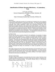
The present analysis compares values of lift coefficient C L , induced drag coefficients C Di and moment<br />
coefficients C m , <strong>for</strong> a range of angle of attack between −2 ◦ and 6 ◦ . The results are shown in Figs. 14, 15<br />
and 16, and an excellent correlation is obtained between the two approaches. For the sake of clarity, the lift<br />
coefficient comparison of Fig. 14 take into account the lift slope given by other theories which are<br />
1. profile wing slope (AR → ∞), a 0 = 2π<br />
2. finite wing slope 37 <strong>for</strong> elliptical lift distribution (Oswald number e = 1), valid <strong>for</strong> small values of sweep<br />
angle.<br />
a 0<br />
a =<br />
1 + a 0 /AR<br />
3. Kuchemann 37 wing slope, which corrects the finite wing slope in the case of non-zero sweep angle Λ.<br />
a =<br />
a 0 cos(Λ)<br />
( √ 1 + z 2 + z)<br />
(73)<br />
where z = a 0 cos(Λ)/(πAR).<br />
As expected the lift coefficients given by the Kuchemann theory, AVL and the vortex lattice under validation<br />
are very well correlated.<br />
For the induced drag coefficient (Fig. 15), again a good correlation can be observed with a maximum<br />
relative error of 7% which corresponds to an angle of attack of 6 ◦ . In terms of moment coefficient, which<br />
is evaluated about the leading edge of the root chord, the maximum relative error is 7% when the angle of<br />
attack is 6 ◦ .<br />
17 of 23<br />
American Institute of Aeronautics and Astronautics
0.7<br />
0.6<br />
0.5<br />
0.4<br />
0.3<br />
CL<br />
0.2<br />
0.1<br />
0<br />
−0.1<br />
−0.2<br />
VL<br />
Kuchemann lift slope<br />
Finite wing slope<br />
Profile slope<br />
AVL<br />
−0.3<br />
−2 −1 0 1 2 3 4 5 6<br />
α [deg]<br />
Figure 14: Lift coefficient vs. angle of attack.<br />
VL<br />
8<br />
9 x 10⁻³ α [deg]<br />
AVL<br />
0.2<br />
VL<br />
7<br />
0.1<br />
AVL<br />
6<br />
0<br />
5<br />
CDi<br />
4<br />
3<br />
Cm<br />
−0.1<br />
−0.2<br />
2<br />
1<br />
−0.3<br />
0<br />
−2 −1 0 1 2 3 4 5 6<br />
−0.4<br />
Figure 15: Induced drag coefficient vs. angle of attack.<br />
−0.5<br />
−2 −1 0 1 2 3 4 5 6<br />
α [deg]<br />
Figure 16: Moment coefficient vs. angle of attack.<br />
V. Aeroelastostatic System<br />
In this section the structural and aerodynamic tools previously developed are linked together, in order<br />
to generate the static aeroelastic system. The aerodynamic loads acting on the wing depend on how the<br />
flow field is affected by the wing geometry. Because the wing is not rigid, the loads acting on the wing<br />
surface induce a de<strong>for</strong>mation of the wing. This change in shape affects the original flow field, leading to a<br />
feedback-loop between aerodynamics and the structure.<br />
V.A.<br />
Generalised Aerodynamic Forces<br />
As seen from section IV the evaluation of the influence coefficients, providing the velocity induced by a<br />
certain horseshoe, is the first step in the calculation of the aerodynamic loads. These quantities are, via the<br />
Biot-Savart law, non-linear functions of the geometry of the wing, and thus of the wing shape. A certain<br />
number of displacements and the direction cosines need to be provided <strong>for</strong> each panel in order to locate and<br />
orientate them in space. Referring to Fig. 11 these quantities correspond to those of the four corners of each<br />
panel (point A,B,E and F) and the orientation structural angles ψ x and ψ y at the control point. In order<br />
to interface aerodynamic and structure the boundary condition in Eq. (68) has to be modified. The normal<br />
to the panel is expressed in global coordinates by means of two successive rotations, namely ψ x about the<br />
local y axis, and φ ∗ = ψ y + φ about the global x axis, where φ is the dihedral angle. Finally the boundary<br />
condition can be expressed in terms of the structural angles as:<br />
w xm sinψ xm − w ym sin ψ xm cosφ ∗ m + w zm cosψ xm cosφ ∗ m = U ∞ (cosφ ∗ m cosψ xm sin α − sinψ xm cosα) (74)<br />
There<strong>for</strong>e, the vector ∆ = [. . . ,u A m ,uB m ,uE m ,uF m , ψ xm , φ∗ m , . . .]T , which collects the displacements needed as<br />
the input to the aerodynamic code, can be defined. Using Eqs. (17) and (18), this vector can be related to<br />
18 of 23<br />
American Institute of Aeronautics and Astronautics
U ∞ 30 m/s<br />
α 3 ( ◦ )<br />
ρ 1.22 kg/m 3<br />
N p 26 -<br />
Table 5: Flow features.<br />
E 1 75.8 GPa<br />
E 2 5.5 GPa<br />
ν 12 0.27 -<br />
G 12 7.2 GPa<br />
ρ 1380 Kg/m 3<br />
Table 6: Kevlar Epoxy main<br />
properties.<br />
E 1 30.3 GPa<br />
E 2 15.9 GPa<br />
ν 12 0.31 -<br />
G 12 5.52 GPa<br />
ρ 4700 Kg/m 3<br />
d 13 4.6 10 −10 m/V<br />
d 23 −2.1 10 −10 m/V<br />
t 0.3 10 −3 m<br />
∆χ 0.5 10 −3 m<br />
Table 7: Macro Fiber Composite<br />
main properties.<br />
Figure 17: Skin and MFC patches web orientation<br />
scheme on the winglet.<br />
Figure 18: Wing box scheme.<br />
the structural generalised coordinates through the matrix G<br />
∆ = G q (75)<br />
Equation (71), which gives the vector containing the vortices on each panel, can be related to the generalised<br />
coordinates<br />
Γ = U ∞ A(∆) −1 b(α) = U ∞ A(G q) −1 b(α) (76)<br />
Finally, using the Kutta-Joukowsky law given by Eq. (72), the aerodynamic <strong>for</strong>ce vector f m on the m-th<br />
panel can be evaluated as a non-linear function of the generalised coordinates. The overall aerodynamic load<br />
distribution on the panels can be regarded as a distribution of concentrated loads. Thus Eq. (55) is applied<br />
in order to evaluate the generalised aerodynamic load vector<br />
e aer (q) =<br />
N p<br />
∑<br />
m=1<br />
S(x m , y m , z m ) T f m (q) (77)<br />
The static solution is given by the equilibrium between the elastic <strong>for</strong>ces, the actuator <strong>for</strong>ces and the<br />
generalised-coordinate-dependent aerodynamic <strong>for</strong>ces<br />
(<br />
K + K<br />
A ) q = e aer (q) + e ext + e V V + e ∆T ∆T (78)<br />
The non-linear system can be solved iteratively via a Newton-Raphson method.<br />
V.B.<br />
A Preliminary Test Case<br />
The effect of piezo-patches actuation on the aerodynamic coefficients is discussed in this section. The wing<br />
under investigation is a 30 ◦ leading edge swept-back, with 0.3 m of aerodynamic chord at the root, taper<br />
19 of 23<br />
American Institute of Aeronautics and Astronautics
CL<br />
0.23<br />
0.225<br />
0.22<br />
Cmac<br />
1.24<br />
1.23<br />
1.22<br />
1.21<br />
1.2<br />
1.19<br />
θ p = 0 ◦<br />
θ p = 15 ◦<br />
θ p = 30 ◦<br />
θ p = 45 ◦<br />
θ p = 60 ◦<br />
θ p = 75 ◦<br />
θ p = 90 ◦<br />
V + = V − =0<br />
0.215<br />
1.18<br />
0 10 20 30 40 50 60 70 80 90<br />
0 10 20 30 40 50 60 70 80 90<br />
θ S θ S<br />
Figure 19: Lift and moment coefficients φ w = 0 ◦ .<br />
CL<br />
0.23<br />
0.225<br />
0.22<br />
Cmac<br />
1.24<br />
1.23<br />
1.22<br />
1.21<br />
1.2<br />
1.19<br />
θ p = 0 ◦<br />
θ p = 15 ◦<br />
θ p = 30 ◦<br />
θ p = 45 ◦<br />
θ p = 60 ◦<br />
θ p = 75 ◦<br />
θ p = 90 ◦<br />
V + = V − =0<br />
0.215<br />
1.18<br />
0 10 20 30 40 50 60 70 80 90<br />
0 10 20 30 40 50 60 70 80 90<br />
θ S θ S<br />
Figure 20: Lift and moment coefficients φ w = 15 ◦ .<br />
ratio 0.33, and 1.9 m of span, b. The wing box has a structural chord that is 50% of the local aerodynamic<br />
chord, while the depth is 7% of it. A hinge placed at 75% of the span, splits the the wing in to an inner<br />
(the baseline) and an outer (the winglet) portion. The hinge angle φ w , and thus the winglet position, can be<br />
varied by means of a torque actuator. A total number of 5 ribs, equally spaced, are placed within the baseline,<br />
while 3 ribs are allocated <strong>for</strong> the winglet. The wing box is entirely realised in Kevlar Epoxy composite (see<br />
Tab. 6). All the ticknesses are set to 1 mm, while the cap areas are set to 25 × 10 −6 m 2 . The wing is set to<br />
fly at a speed of U ∞ = 30 m/s and at an angle of attack α = 3 ◦ . The aerodynamic loads are based on 10<br />
panels <strong>for</strong> inner wing and 6 on the outer. The flow features are given in Tab. 5. An overall structural and<br />
aerodynamic symmetry condition about the x-z plane is assumed.<br />
A type of piezoceramic composite actuator commonly known as the Macro Fiber Composite (MFC) actuator<br />
is used <strong>for</strong> the present simulations. The MFC actuator, developed at NASA Langley Research Center, 42<br />
is a layered, planar actuation device that employs rectangular cross-section, unidirectional piezoceramic<br />
fibers (PZT 5A) embedded in a thermosetting polymer matrix. This active, fiber rein<strong>for</strong>ced layer is then<br />
sandwiched between copper-clad Kapton film layers that have an etched interdigitated electrode pattern.<br />
Because of the in-plane poling the MFC uses the d 33 piezoelectric effect, which is much stronger than the d 31<br />
effect used by traditional PZT actuators with through-the-thickness poling. The theory developed in Sec. III<br />
can be easily extended to the case of MFC patches simply considering, as voltage actuation input parameter<br />
V/t, the distance between the in-plane electrodes ∆χ in place of the patch thickness t. The MFC patches<br />
work in a voltage range of -500 to 1500 V and the main parameters are given in Tab. 7. 43 Implementation<br />
of MFC patches <strong>for</strong> the control of a small manned aircraft has been successfully done by Bilgen et al. 4<br />
A total number of four MFC patches of dimension 0.056×0.085 m, are placed on the winglet. Specifiacally,<br />
two of them are placed on the upper surface, along the elastic axis direction, and loaded with the maximum<br />
positive voltage of 1500 V; the other two are placed on the lower skin and loaded with the maximum negative<br />
voltage -500 V. The goal is to investigate the effect of the skin and piezo-patches composite-web orientations,<br />
identified by the angles θ s and θ p respectively, on the aerodynamic coefficients. The local material coordinate<br />
system of the skin and the piezo-patches are given in Fig. 17, while a scheme of the whole configuration<br />
20 of 23<br />
American Institute of Aeronautics and Astronautics
is given in Fig. 18. Moreover, two winglet configurations will be analysed, namely the unfolded winglet<br />
with φ w = 0 ◦ and winglet folded upwards at φ w = 15 ◦ . For these two cases, the aerodynamic coefficients of<br />
the whole flying wing are evaluated with respect to the same reference length, namely the wing span of the<br />
unfolded configuration.<br />
Results from the simulations are given in Figs. 19 and 20 <strong>for</strong> the φ w = 0 ◦ and φ w = 15 ◦ case respectively,<br />
where the aerodynamic coefficient C L and the pitching moment coefficient C mac about the aerodynamic<br />
centre, are given as a function of θ s and θ p . Moreover, the values of the coefficients evaluated when no voltage<br />
input is given to the patches, are set to be reference values in each diagram. These reference coefficients,<br />
which are due only to the fluid-structure interaction, are minimally affected by the composite web angles,<br />
and thus are evaluated as the mean value over the θ s and θ p domain. The results can be summarised as<br />
follows:<br />
• <strong>for</strong> θ s = 37 ◦ and θ p = 0 ◦ the maximum positive variation occurs <strong>for</strong> both the folded and the unfolded<br />
configurations (see Tab. 8); this combination of angles causes the winglet to twist with a positive angle,<br />
and thus to increase the local angle of attack. The displacement field relative to the unfolded case, is<br />
given in Fig. 21.<br />
• <strong>for</strong> θ s = 30 ◦ and θ p = 90 ◦ the maximum negative variation occurs <strong>for</strong> both the folded and the unfolded<br />
configuration (see Tab. 9); the winglet undergoes to a negative torsion that decreases the local angle<br />
of attack. The displacement field relative to the unfolded case, is given in Fig. 22.<br />
φ w [ ◦ ] ∆C L [%] ∆C Di [%] ∆C mac [%]<br />
0 3.06 7.65 2.27<br />
15 3.12 7.90 2.31<br />
Table 8: Aerodynamic coefficients variation <strong>for</strong><br />
θ s = 37 ◦ and θ p = 0 ◦ .<br />
φ w [ ◦ ] ∆C L [%] ∆C Di [%] ∆C mac [%]<br />
0 -1.50 -2.50 -1.12<br />
15 -1.55 -2.74 -1.32<br />
Table 9: Aerodynamic coefficients variation <strong>for</strong><br />
θ s = 30 ◦ and θ p = 90 ◦ .<br />
x 10 −3<br />
x 10 −3<br />
5<br />
3<br />
0.2<br />
0.2<br />
2.8<br />
0.15<br />
4.5<br />
0.15<br />
2.6<br />
2.4<br />
y [m]<br />
0.1<br />
4<br />
3.5<br />
y [m]<br />
0.1<br />
2.2<br />
2<br />
1.8<br />
0.05<br />
3<br />
0.05<br />
1.6<br />
0<br />
0.05 0.1 0.15 0.2<br />
x [m]<br />
Figure 21: Winglet displacement field: θ s = 37 ◦ ,<br />
θ p = 0 ◦ and φ w = 0 ◦ .<br />
0<br />
0.05 0.1 0.15 0.2<br />
x [m]<br />
Figure 22: Winglet displacement field: θ s = 30 ◦ ,<br />
θ p = 90 ◦ and φ w = 0 ◦ .<br />
1.4<br />
VI. Concluding Remarks<br />
The paper presents a computational approach <strong>for</strong> a parameterized static aeroelastic model, addressed to<br />
preliminary conceptual design of morphing aircraft. The approach relies on a continuum modeling based on<br />
an equivalent plate model approach <strong>for</strong> the structural modeling, a subsonic quasi-static 3D vortex lattice<br />
method <strong>for</strong> the aerodynamic load, and actuation modeling based on strain actuation: validation of the<br />
models are provided at each step. Finally an example of the capability of the code has been given.<br />
Once the aeroelastic model proposed is set up several options are possible in order to investigate morphing<br />
via a distribution of actuation; an optimisation algorithm, such as a genetic algorithm (GA), can be<br />
implemented to find the best combination of composite material orientation, wing geometry and actuator<br />
positions which minimises the energy required to achieve a certain wing shape, thus a certain manoeuvre. It<br />
is also possible to consider other cost functions such as the lift to drag ratio. In order to deal with aeroelastic<br />
21 of 23<br />
American Institute of Aeronautics and Astronautics
esponse problems an unsteady aerodynamic code needs to be implemented: the choice can rely either on a<br />
simple 2D Theodorsen strip method, as a first step, or on more sophisticated 3D unsteady panel methods.<br />
Finally the actuation scenario can be extended in order to include point-to-point truss-actuators.<br />
Acknowledgments<br />
This work has been supported by a Marie-Curie excellence research grant funded by the European<br />
Commission, and by a WUN (Worldwide University Network).<br />
References<br />
1 D. Voracek, E. Pendleton and E. K. Griffin, “The Active Aeroelastic Wing Phase I Flight Research Through”, NASA/TM-<br />
2003-210741.<br />
2 de Marmier, P. and Wereley, N., “<strong>Morphing</strong> Wings of a Small Scale UAV Using inflatable Actuators <strong>for</strong> Sweep Control”,<br />
44th AIAA/ASME/ASCE/AHS/ASC Structures, Structural Dynamics and Materials Conference, 2003, pp. 110, AIAA-2003-<br />
1802.<br />
3 O. Bilgen, K. Kochersberger, E. C. Diggs, A. J. Kurdila, D. J. Inman, “<strong>Morphing</strong> Wing Micro-Air-Vehicles via Macro-Fiber-<br />
Composite Actuators”, 48th AIAA/ASME/ASCE/AHS/ASC Structures, Structural Dynamics, and Materials Conference, 23<br />
- 26 April 2007, Honolulu, Hawaii, AIAA 2007-1785.<br />
4 O. Bilgen, K. Kochersberger, E. C. Diggs, A. J. Kurdila, D. J. Inman, “<strong>Morphing</strong> Wing Aerodynamic Control via Macro-<br />
Fiber-Composite Actuators in an Unmanned <strong>Aircraft</strong>”, AIAA 2007 Conference and Exhibit, 7 - 10 May 2007, Rohnert Park,<br />
Cali<strong>for</strong>nia, AIAA 2007-2741.<br />
5 M. R. Schultz, M. W. Hyer, “A <strong>Morphing</strong> Concept Based on Unsymmetric Composite Laminates and Piezoceramic MFC<br />
Actuators”, 45th AIAA/ASME/ASCE/AHS/ASC Structures, Structural Dynamics & Materials Conference, 19 - 22 April<br />
2004, Palm Springs, Cali<strong>for</strong>nia. AIAA 2004-1806.<br />
6 D. T. Grant, M. Abdulrahimy and R. Lindz. “Flight Dynamics of a <strong>Morphing</strong> <strong>Aircraft</strong> Utilizing Independent Multiple-<br />
Joint Wing Sweep”, AIAA Atmospheric Flight Mechanics Conference and Exhibit, 21 - 24 August 2006, Keystone, Colorado.<br />
AIAA 2006-6505.<br />
7 J. N. Scarlett, R. A. Canfield and B. Sanders. “Multibody Dynamic Aeroelastic Simulation of a Folding Wing <strong>Aircraft</strong>”,<br />
47th AIAA/ASME/ASCE/AHS/ASC Structures, Structural Dynamics, and Materials Conference, Newport, Rhode Island.<br />
AIAA 2006-2135.<br />
8 D. A. Neal III, J. Farmer, D. Inman. “Development of a <strong>Morphing</strong> <strong>Aircraft</strong> Model <strong>for</strong> Wind Tunnel Experimentation”, 47th<br />
AIAA/ASME/ASCE/AHS/ASC Structures, Structural Dynamics, and Materials Confere, 1 - 4 May 2006, Newport, Rhode<br />
Island. AIAA 2006-2141.<br />
9 J. S. Bae, T. M. Seigler and D. J. Inman. “Aerodynamic and Static Aeroelastic Characteristics of a Variable-Span <strong>Morphing</strong><br />
Wing”, Journal of <strong>Aircraft</strong>, Vol. 42, No. 2, MarchApril 2005.<br />
10 J. E. Blondeau and D. J. Pines. “Design and Testing of a Pneumatic Telescopic Wing <strong>for</strong> Unmanned Aerial Vehicles”,<br />
Journal of <strong>Aircraft</strong>, Vol. 44, No. 4, JulyAugust 2007.<br />
11 P. Bourdin, A. Gatto, M.I. <strong>Friswell</strong>. “The Application of Variable Cant Angle Winglets <strong>for</strong> <strong>Morphing</strong> <strong>Aircraft</strong> control”,<br />
24th Applied Aerodynamics Conference, San Francisco, Cali<strong>for</strong>nia AIAA paper 2006-3660.<br />
12 N. Ameri, M. H. Lowenberg and M.I. <strong>Friswell</strong>. “<strong>Modelling</strong> the Dynamic Response of a <strong>Morphing</strong> Wing with Active<br />
Winglets”, AIAA Atmospheric Flight Mechanics Conference and Exhibit 20 - 23 August 2007, Hilton Head, South Carolina,<br />
AIAA 2007-6500.<br />
13 A. E. Lovejoy, and R. K. Kapania, “Natural Frequencies and Atlas of Mode Shapes <strong>for</strong> Generally-Laminated, Thick,<br />
Skew, Trapezoidal Plates”, CCMS(Center <strong>for</strong> Composite Materials and Structures)-94-09, Virginia Polytechnic Institute and<br />
State University, Blacksburg, VA, Aug. 1994.<br />
14 “Natural Frequencies and Atlas of Mode Shapes <strong>for</strong> Generally-Laminated, Thick, Skew, Trapezoidal Plates”, MS Thesis,<br />
Department of Aerospace and Ocean Engineering, Virginia Polytechnic Institute and State University, Blacksburg, VA, Aug.<br />
1994.<br />
15 J. N. Reddy and A. Miravete, “Practical Analysis of Composite Laminates”, CRC Press, Inc., Boca Raton, 1995, pp.<br />
52-62.<br />
16 D. J. Dawe , “Buckling and Vibration of Plate Structures Including Shear De<strong>for</strong>mation and Related Effects”, Aspects of<br />
the Analysis of Plate Structures, Ed. by Dawe, D. J., Horsington, R. W., Kamtekar, A. G. and Little, G. H., New York, Ox<strong>for</strong>d<br />
University Press, 1985, pp. 75-99.<br />
17 E. Reissner, “The Effect of Transverse Shear De<strong>for</strong>mation on the Bending of Elastic Plates”, Journal of Applied Mechanics,<br />
Vol. 12, 1945, pp. A-69 77.<br />
18 R. D. Mindlin , “Influence of Rotatory Inertia and Shear on Flexural Motions of Isotropic, Elastic Plates”, Journal of<br />
Applied Mechanics, Vol. 18, 1951, pp. 31-38.<br />
19 R. K. Kapania and S. Raciti, “Recent Advances in Analysis of Laminated Beams and Plates, Part I: Shear Effects and<br />
Buckling”, AIAA Journal, Vol. 27, No. 7, 1989, pp. 923-934.<br />
20 G. L. Giles, “Equivalent Plate Analysis of <strong>Aircraft</strong> Wing Box Structures with General Plan<strong>for</strong>m Geometry”, Journal of<br />
<strong>Aircraft</strong>, Vol. 23, No. 11, 1986, pp. 859-864.<br />
21 G. L. Giles, “Equivalent Plate Modeling <strong>for</strong> Conceptual Design of <strong>Aircraft</strong> Wing Structures”, AIAA Paper 95-3945,<br />
September 1995.<br />
22 of 23<br />
American Institute of Aeronautics and Astronautics
22 S. Tizzi, “Numerical Procedure <strong>for</strong> the Dynamic Analysis of Three-Dimensional Aeronautical Structures”, Journal of<br />
<strong>Aircraft</strong>, Vol. 34, No. 1, 1997, pp. 120-130.<br />
23 E. Livne, “Equivalent Plate Structural Modeling <strong>for</strong> Wing Shape Optimization Including Transverse Shear”, AIAA<br />
Journal, Vol. 32, No. 6, 1994, pp. 1278-1288.<br />
24 E. Livne and I. Navarro, “Nonlinear Equivalent Plate Modeling of Wing Box Structures”, 40th<br />
AIAA/ASME/ASCE/AHS/ASC SDM Conference, April 12-15, 1999, St. Louis, MO, pp. 346-372. Also Journal of<br />
<strong>Aircraft</strong>, Vol. 36, No. 5, 1999, pp. 851-865.<br />
25 R. K. Kapania, and S. Singhvi, “Free Vibration Analyses of Generally Laminated Tapered Skew Plates’,’ Composites<br />
Engineering, Vol. 2, No. 3, 1992, pp. 197212.<br />
26 S. Singhvi, “Analysis, Shape Sensitivities and Approximations of Modal Response of Generally Laminated Tapered Skew<br />
Plates”, M.S. Thesis, Dept. of Aerospace and Ocean Engineering, Virginia Polytechnic Inst. and State Univ., Blacksburg, VA,<br />
Sept. 1991.<br />
27 R. K. Kapania, and A. E. Lovejoy, “Free Vibration of Thick Generally Laminated Cantilever Quadrilateral Plates”, AIAA<br />
Journal, Vol. 34, No. 7, 1996, pp. 14761486; also AIAA Paper 95-1350, 1995.<br />
28 R. K. Kapania, and A. E. Lovejoy, “Free Vibration of Thick Generally Laminated Quadrilateral Plates with Point<br />
Supports”, Journal of <strong>Aircraft</strong>, Vol. 35, No. 6, 1998, pp. 958965; also AIAA Paper 96-1346, 1996.<br />
29 F. Cortial, “Sensitivity of Aeroelastic ResponseofWingsUsingEquivalent Plate Models”, Dept. of Aerospace and Ocean<br />
Engineering,TR,Virginia Polytechnic Inst. and State Univ., Backsburg, VA, 1996.<br />
30 R. K. Kapania and Y. Liu, “Static and Vibration Analyses of General Wing Structures Using Equivalent-Plate Models”,<br />
AIAA Journal, Vol. 38, No. 7, July 2000, Virginia Polytechnic Institute and State University, Blacksburg, Virginia 24061.<br />
31 F. H. Gern, D. J. Inman and R. K. Kapania. “Computation Power Requirements <strong>for</strong> Smart Wings with <strong>Morphing</strong> airfoils”,<br />
AIAA Journal, Vol. 43, No. 12, December 2005.<br />
32 I. Lottati, “Flutter and Divergence Aeroelastic Characteristics <strong>for</strong> composite Forward swept Cantilevered Wings“, Journal<br />
of <strong>Aircraft</strong>, Vol. 22, No. 11, 1985, pp. 1001-1007.<br />
33 L. Librescu, J. Simovich, “A General Formulation <strong>for</strong> the Aeroelastic Divergence of Composite Swept Forward Wing<br />
Structures”Journal of <strong>Aircraft</strong>, Vol. 252, No. 4, 1988, pp. 364-371.<br />
34 L. Demasi and E. Livne, “Structural Ritz-Based Simple-Polynomials Nonlinear Equivalent Plate Approach - An Assessment”,<br />
46th AIAA/ASME/ASCE/AHS/ASC Conference, April 18-21, 2005, Austin, Texas, AIAA 2005-2093.<br />
35 F. Cote’ ,P. Masson, N. Mrad, V. Cotoni, “Dynamic and static modelling of piezoelectric composite structures using a<br />
thermal analogy with MSC/NASTRAN”, Composite Structures 65 (2004) 471484.<br />
36 E. J., “Barbero Introduction to Composite Material Design”. Taylor & Francis .<br />
37 J. D. Anderson, “Fundamentals of Aerodynamics”, McGraw-Hill, 1991.<br />
38 J. J. Bertin, “Aerodynamics <strong>for</strong> Engineers”, fourth edition.<br />
39 J. Katz, A. Plotkin, “Low-Speed Aerodynamics”.<br />
40 P. G. Saffman, “Vortex Dynamics” Cambridge Univeristy press.<br />
41 http://web.mit.edu/drela/Public/web/avl/ - 01/08.<br />
42 W. K. Wilkie, G. R. Bryant, J. W. High,, “Low-Cost Piezocomposite Actuator <strong>for</strong> Structural Control Applications”,<br />
SPIE 7th Annual International Symposium on Smart Structures and Materials, Newport Beach, CA, 2000.<br />
43 www.smart-material.com<br />
23 of 23<br />
American Institute of Aeronautics and Astronautics