Modelling Continuously Morphing Aircraft for ... - Michael I Friswell

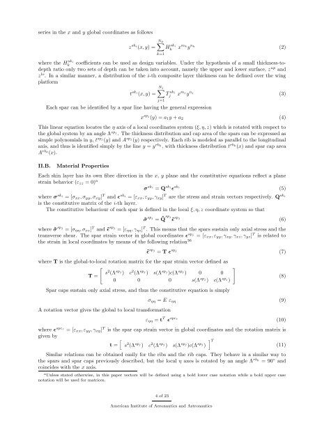
series in the x and y global coordinates as follows
∑N k
z ski (x, y) = H ski
k
x m k
y n k
(2)
k=1
where the H ski
k
coefficients can be used as design variables. Under the hypothesis of a small thickness-todepth
ratio only two sets of depth can be taken into account, namely the upper and lower surface, z up and
z lo . In a similar manner, a distribution of the i-th composite layer thickness can be defined over the wing
platform
N
∑ j
t ski (x, y) = T ski
j
x mj y nj (3)
Each spar can be identified by a spar line having the general expression
j=1
x spj (y) = a 1 y + a 2 (4)
This linear equation locates the η axis of a local coordinates system (ξ, η, z) which is rotated with respect to
the global system by an angle Λ spj . The thickness distribution and cap area of the spars can be expressed as
simple polynomials in y, t spj (y) and A spj (y) respectively. Each rib is modeled as parallel to the longitudinal
axis, and thus is identified simply by the line y = y rb k
, with thickness distribution t rb k
(x) and spar cap area
A rb k
(x).
II.B. Material Properties
Each skin layer has its own fibre direction in the x, y plane and the constitutive equations reflect a plane
strain behavior (ε zz = 0) a σ ski = Q ski ǫ ski (5)
where σ ski = [σ xx , σ yy , σ xy ] T and ǫ ski = [ε xx , ε yy , γ xy ] T are the stress and strain vectors respectively. Q ski
is the constitutive matrix of the i-th layer.
The constitutive behaviour of each spar is defined in the local ξ, η, z coordinate system so that
˜σ spj = ˜Q spj˜ǫ spj (6)
where ˜σ spj = [σ ηη , σ xz ] T and ˜ǫ spj = [ε ηη , γ ηz ] T . This means that the spars sustain only axial stress and the
transverse shear. The spar strain vector in global coordinates ǫ spj = [ε xx , ε yy , γ xy , γ xz , γ yz ] T is related to
the strain in local coordinates by means of the following relation 36
˜ǫ spj = T ǫ spj (7)
where T is the global-to-local rotation matrix for the spar strain vector defined as
[
]
s
T =
2 (Λ spj ) c 2 (Λ spj ) s(Λ spj )c(Λ spj ) 0 0
0 0 0 s(Λ spj ) c(Λ spj )
Spar caps sustain only axial stress, and thus the constitutive equation is simply
A rotation vector gives the global to local transformation
σ ηη = E ε ηη (9)
ε ηη = t T ǫ spcr (10)
where ǫ spcr = [ε xx , ε yy , γ xy ] T is the spar cap strain vector in global coordinates and the rotation matrix is
given by
[
] T
t = s 2 (Λ spj ) c 2 (Λ spj ) s(Λ spj )c(Λ spj )
(11)
Similar relations can be obtained easily for the ribs and the rib caps. They behave in a similar way to
the spars and spar caps previously described, but the local η axes is rotated by an angle Λ rb k
= 90 ◦ and
coincides with the x axis.
a Unless stated otherwise, in this paper vectors will be defined using a bold lower case notation while a bold upper case
notation will be used for matrices.
(8)
4 of 23
American Institute of Aeronautics and Astronautics