- Page 1 and 2:
Phenomena Second Edition ,cro о Ma
- Page 4 and 5:
Transport Phenomena Second Edition
- Page 6 and 7:
Preface While momentum, heat, and m
- Page 8 and 9:
Contents Preface Chapter 0 The Subj
- Page 10 and 11:
Contents vii Ex. 8.3-3 Tangential A
- Page 12 and 13:
Contents ix Ex. 15.5-1 Heating of a
- Page 14 and 15:
Contents xi §22.7° Effects of Int
- Page 16 and 17:
Chapter 0 The Subject of Transport
- Page 18 and 19:
§0.2 Three Levels At Which Transpo
- Page 20 and 21:
§0.3 The Conservation Laws: An Exa
- Page 22 and 23:
§0.4 Concluding Comments 7 The con
- Page 24:
Part One Momentum Transport
- Page 27 and 28:
12 Chapter 1 Viscosity and the Mech
- Page 29 and 30:
14 Chapter 1 Viscosity and the Mech
- Page 31 and 32:
16 Chapter 1 Viscosity and the Mech
- Page 33 and 34:
18 Chapter 1 Viscosity and the Mech
- Page 35 and 36:
20 Chapter 1 Viscosity and the Mech
- Page 37 and 38:
22 Chapter 1 Viscosity and the Mech
- Page 39 and 40:
24 Chapter 1 Viscosity and the Mech
- Page 41 and 42:
26 Chapter 1 Viscosity and the Mech
- Page 43 and 44:
28 Chapter 1 Viscosity and the Mech
- Page 45 and 46:
30 Chapter 1 Viscosity and the Mech
- Page 47 and 48:
32 Chapter 1 Viscosity and the Mech
- Page 49 and 50:
34 Chapter 1 Viscosity and the Mech
- Page 51 and 52:
36 Chapter 1 Viscosity and the Mech
- Page 53 and 54:
38 Chapter 1 Viscosity and the Mech
- Page 55 and 56:
Chapter 2 Shell Momentum Balances a
- Page 57 and 58:
42 Chapter 2 Shell Momentum Balance
- Page 59 and 60:
44 Chapter 2 Shell Momentum Balance
- Page 61 and 62:
46 Chapter 2 Shell Momentum Balance
- Page 63 and 64:
48 Chapter 2 Shell Momentum Balance
- Page 65 and 66:
50 Chapter 2 Shell Momentum Balance
- Page 67 and 68:
52 Chapter 2 Shell Momentum Balance
- Page 69 and 70:
54 Chapter 2 Shell Momentum Balance
- Page 71 and 72:
56 Chapter 2 Shell Momentum Balance
- Page 73 and 74:
58 Chapter 2 Shell Momentum Balance
- Page 75 and 76:
60 Chapter 2 Shell Momentum Balance
- Page 77 and 78:
62 Chapter 2 Shell Momentum Balance
- Page 79 and 80:
64 Chapter 2 Shell Momentum Balance
- Page 81 and 82:
66 Chapter 2 Shell Momentum Balance
- Page 83 and 84:
68 Chapter 2 Shell Momentum Balance
- Page 85 and 86:
70 Chapter 2 Shell Momentum Balance
- Page 87 and 88:
72 Chapter 2 Shell Momentum Balance
- Page 89 and 90:
74 Chapter 2 Shell Momentum Balance
- Page 91 and 92: 76 Chapter 3 The Equations of Chang
- Page 93 and 94: 78 Chapter 3 The Equations of Chang
- Page 95 and 96: 80 Chapter 3 The Equations of Chang
- Page 97 and 98: 82 Chapter 3 The Equations of Chang
- Page 99 and 100: 84 Chapter 3 The Equations of Chang
- Page 101 and 102: 86 Chapter 3 The Equations of Chang
- Page 103 and 104: 88 Chapter 3 The Equations of Chang
- Page 105 and 106: 90 Chapter 3 The Equations of Chang
- Page 107 and 108: 92 Chapter 3 The Equations of Chang
- Page 109 and 110: 94 Chapter 3 The Equations of Chang
- Page 111 and 112: 96 Chapter 3 The Equations of Chang
- Page 113 and 114: 98 Chapter 3 The Equations of Chang
- Page 115 and 116: 100 Chapter 3 The Equations of Chan
- Page 117 and 118: 102 Chapter 3 The Equations of Chan
- Page 119 and 120: 104 Chapter 3 The Equations of Chan
- Page 121 and 122: 106 Chapter 3 The Equations of Chan
- Page 123 and 124: 108 Chapter 3 The Equations of Chan
- Page 125 and 126: 110 Chapter 3 The Equations of Chan
- Page 127 and 128: 112 Chapter 3 The Equations of Chan
- Page 129 and 130: Chapter 4 Velocity Distributions wi
- Page 131 and 132: 116 Chapter 4 Velocity Distribution
- Page 133 and 134: 118 Chapter 4 Velocity Distribution
- Page 135 and 136: 120 Chapter 4 Velocity Distribution
- Page 137 and 138: 122 Chapter 4 Velocity Distribution
- Page 139 and 140: 124 Chapter 4 Velocity Distribution
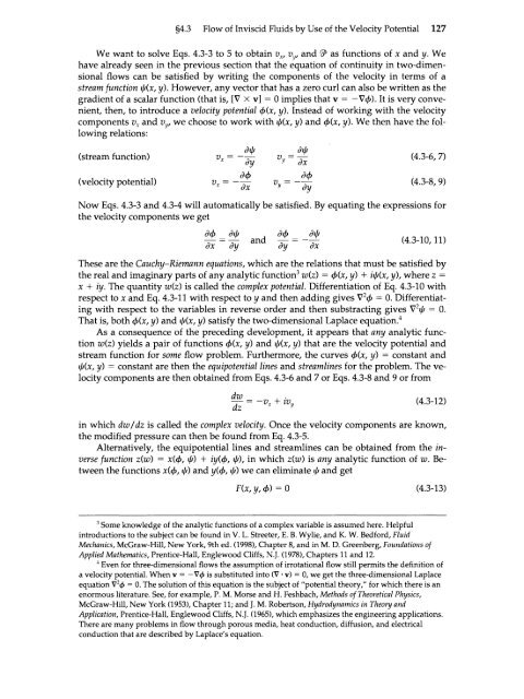
- Page 141: 126 Chapter 4 Velocity Distribution
- Page 145 and 146: 130 Chapter 4 Velocity Distribution
- Page 147 and 148: 132 Chapter 4 Velocity Distribution
- Page 149 and 150: 134 Chapter 4 Velocity Distribution
- Page 151 and 152: 136 Chapter 4 Velocity Distribution
- Page 153 and 154: 138 Chapter 4 Velocity Distribution
- Page 155 and 156: 140 Chapter 4 Velocity Distribution
- Page 157 and 158: 142 Chapter 4 Velocity Distribution
- Page 159 and 160: 144 Chapter 4 Velocity Distribution
- Page 161 and 162: 146 Chapter 4 Velocity Distribution
- Page 163 and 164: 148 Chapter 4 Velocity Distribution
- Page 165 and 166: 150 Chapter 4 Velocity Distribution
- Page 167 and 168: Chapter 5 Velocity Distributions in
- Page 169 and 170: 154 Chapter 5 Velocity Distribution
- Page 171 and 172: 156 Chapter 5 Velocity Distribution
- Page 173 and 174: 158 Chapter 5 Velocity Distribution
- Page 175 and 176: 160 Chapter 5 Velocity Distribution
- Page 177 and 178: 162 Chapter 5 Velocity Distribution
- Page 179 and 180: 164 Chapter 5 Velocity Distribution
- Page 181 and 182: 166 Chapter 5 Velocity Distribution
- Page 183 and 184: 168 Chapter 5 Velocity Distribution
- Page 185 and 186: 170 Chapter 5 Velocity Distribution
- Page 187 and 188: 172 Chapter 5 Velocity Distribution
- Page 189 and 190: 174 Chapter 5 Velocity Distribution
- Page 191 and 192: 176 Chapter 5 Velocity Distribution
- Page 193 and 194:
178 Chapter 6 Interphase Transport
- Page 195 and 196:
180 Chapter 6 Interphase Transport
- Page 197 and 198:
1 182 Chapter 6 Interphase Transpor
- Page 199 and 200:
184 Chapter 6 Interphase Transport
- Page 201 and 202:
186 Chapter 6 Interphase Transport
- Page 203 and 204:
188 Chapter 6 Interphase Transport
- Page 205 and 206:
190 Chapter 6 Interphase Transport
- Page 207 and 208:
192 Chapter 6 Interphase Transport
- Page 209 and 210:
194 Chapter 6 Interphase Transport
- Page 211 and 212:
196 Chapter 6 Interphase Transport
- Page 213 and 214:
198 Chapter 7 Macroscopic Balances
- Page 215 and 216:
200 Chapter 7 Macroscopic Balances
- Page 217 and 218:
202 Chapter 7 Macroscopic Balances
- Page 219 and 220:
204 Chapter 7 Macroscopic Balances
- Page 221 and 222:
206 Chapter 7 Macroscopic Balances
- Page 223 and 224:
208 Chapter 7 Macroscopic Balances
- Page 225 and 226:
210 Chapter 7 Macroscopic Balances
- Page 227 and 228:
212 Chapter 7 Macroscopic Balances
- Page 229 and 230:
214 Chapter 7 Macroscopic Balances
- Page 231 and 232:
216 Chapter 7 Macroscopic Balances
- Page 233 and 234:
218 Chapter 7 Macroscopic Balances
- Page 235 and 236:
220 Chapter 7 Macroscopic Balances
- Page 237 and 238:
222 Chapter 7 Macroscopic Balances
- Page 239 and 240:
•< 224 Chapter 7 Macroscopic Bala
- Page 241 and 242:
226 Chapter 7 Macroscopic Balances
- Page 243 and 244:
228 Chapter 7 Macroscopic Balances
- Page 245 and 246:
230 Chapter 7 Macroscopic Balances
- Page 247 and 248:
232 Chapter 8 Polymeric Liquids onl
- Page 249 and 250:
234 Chapter 8 Polymeric Liquids is,
- Page 251 and 252:
236 Chapter 8 Polymeric Liquids Fig
- Page 253 and 254:
238 Chapter 8 Polymeric Liquids Upp
- Page 255 and 256:
240 Chapter 8 Polymeric Liquids о
- Page 257 and 258:
242 Chapter 8 Polymeric Liquids Tab
- Page 259 and 260:
244 Chapter 8 Polymeric Liquids EXA
- Page 261 and 262:
246 Chapter 8 Polymeric Liquids Thi
- Page 263 and 264:
248 Chapter 8 Polymeric Liquids EXA
- Page 265 and 266:
250 Chapter 8 Polymeric Liquids bet
- Page 267 and 268:
252 Chapter 8 Polymeric Liquids (b)
- Page 269 and 270:
254 Chapter 8 Polymeric Liquids Fig
- Page 271 and 272:
256 Chapter 8 Polymeric Liquids 10,
- Page 273 and 274:
258 Chapter 8 Polymeric Liquids QUE
- Page 275 and 276:
260 Chapter 8 Polymeric Liquids The
- Page 277 and 278:
262 Chapter 8 Polymeric Liquids 8C.
- Page 280 and 281:
Thermal Conductivity and the Mechan
- Page 282 and 283:
§9.1 Fourier's Law of Heat Conduct
- Page 284 and 285:
§9.1 Fourier's Law of Heat Conduct
- Page 286 and 287:
Table 9.1-4 Thermal Conductivities,
- Page 288 and 289:
§9.2 Temperature and Pressure Depe
- Page 290 and 291:
§9.3 Theory of Thermal Conductivit
- Page 292 and 293:
§9.3 Theory of Thermal Conductivit
- Page 294 and 295:
§9.4 THEORY OF THERMAL CONDUCTIVIT
- Page 296 and 297:
§9.6 Effective Thermal Conductivit
- Page 298 and 299:
§9.7 Convective Transport of Energ
- Page 300 and 301:
§9.8 Work Associated with Molecula
- Page 302 and 303:
Problems 287 9A.1 Prediction of the
- Page 304 and 305:
Problems 289 mated as oblate sphero
- Page 306 and 307:
§10.1 Shell Energy Balances; Bound
- Page 308 and 309:
§10.2 Heat Conduction with an Elec
- Page 310 and 311:
§10.2 Heat Conduction with an Elec
- Page 312 and 313:
§10.3 Heat Conduction with a Nucle
- Page 314 and 315:
§10.4 Heat Conduction with a Visco
- Page 316 and 317:
§10.5 Heat Conduction with a Chemi
- Page 318 and 319:
§10.6 Heat Conduction Through Comp
- Page 320 and 321:
§10.6 Heat Conduction Through Comp
- Page 322 and 323:
§10.7 Heat Conduction in a Cooling
- Page 324 and 325:
§10.7 Heat Conduction in a Cooling
- Page 326 and 327:
§10.8 Forced Convection 311 Forced
- Page 328 and 329:
§10.8 Forced Convection 313 term c
- Page 330 and 331:
§10.8 Forced Convection 315 Unifor
- Page 332 and 333:
§10.9 Free Convection 317 fluid in
- Page 334 and 335:
Questions for Discussion 319 The ve
- Page 336 and 337:
Problems 321 1 3 = V "T 2 = 61 °F
- Page 338 and 339:
Problems 323 Fig. 10B.4. Temperatur
- Page 340 and 341:
Problems 325 - T a ) Answer: P =
- Page 342 and 343:
Problems 327 the temperatures at th
- Page 344 and 345:
Problems 329 Zone II in which heat
- Page 346 and 347:
Problems 331 (a) Show that the diff
- Page 348 and 349:
Nonisothermal Systems §11.1 The en
- Page 350 and 351:
§11.1 The Energy Equation 335 disi
- Page 352 and 353:
§11.2 Special Forms of the Energy
- Page 354 and 355:
§11.4 Use of the Equations of Chan
- Page 356 and 357:
Cont. — |p=-(V-pv) 3.1-4 For p =
- Page 358 and 359:
§11.4 Use of the Equations of Chan
- Page 360 and 361:
§11.4 Use of the Equations of Chan
- Page 362 and 363:
§11Л Use of the Equations of Chan
- Page 364 and 365:
§11.4 Use of the Equations of Chan
- Page 366 and 367:
§11.4 Use of the Equations of Chan
- Page 368 and 369:
§11.5 Dimensional Analysis of the
- Page 370 and 371:
§11.5 Dimensional Analysis of the
- Page 372 and 373:
§11.5 Dimensional Analysis of the
- Page 374 and 375:
§11.5 Dimensional Analysis of the
- Page 376 and 377:
Problems 361 In principle, we may s
- Page 378 and 379:
Problems 363 for methane are: a = 2
- Page 380 and 381:
Problems 365 11B.6. Transpiration c
- Page 382 and 383:
Problems 367 examined. The wax drop
- Page 384 and 385:
Problems 369 (b) Choose appropriate
- Page 386 and 387:
Problems 371 (a) For the "true" sys
- Page 388 and 389:
Problems 373 The first term on the
- Page 390 and 391:
§12.1 Unsteady Heat Conduction in
- Page 392 and 393:
§12.1 Unsteady Heat Conduction in
- Page 394 and 395:
§12.1 Unsteady Heat Conduction in
- Page 396 and 397:
§12.2 Steady Heat Conduction in La
- Page 398 and 399:
§12.2 Steady Heat Conduction in La
- Page 400 and 401:
§12.3 Steady Potential Flow of Hea
- Page 402 and 403:
§12.4 Boundary Layer Theory for No
- Page 404 and 405:
§12.4 Boundary Layer Theory for No
- Page 406 and 407:
§12.4 Boundary Layer Theory for No
- Page 408 and 409:
§12.4 Boundary Layer Theory for No
- Page 410 and 411:
Problems 395 PROBLEMS 12A.1. Unstea
- Page 412 and 413:
Problems 397 (d) Then solve the equ
- Page 414 and 415:
Problems 399 Fluid approaches with
- Page 416 and 417:
Problems 401 in which a 0 = k o /pC
- Page 418 and 419:
Problems 403 themselves at a reason
- Page 420 and 421:
Problems 405 (d) Obtain the lowest
- Page 422 and 423:
§13.1 Time-smoothed equations of c
- Page 424 and 425:
§13.2 The Time-Smoothed Temperatur
- Page 426 and 427:
§13.4 Temperature Distribution for
- Page 428 and 429:
§13.4 Temperature Distribution for
- Page 430 and 431:
§13.5 TEMPERATURE DISTRIBUTION FOR
- Page 432 and 433:
§13.6 Fourier Analysis of Energy T
- Page 434 and 435:
§13.6 Fourier Analysis of Energy T
- Page 436 and 437:
Sh ReSc 1/3 Vf/2 Problems 421 = 0.0
- Page 438 and 439:
§14.1 Definitions of Heat Transfer
- Page 440 and 441:
§14.1 Definitions of Heat Transfer
- Page 442 and 443:
§14.1 Definitions of Heat Transfer
- Page 444 and 445:
§14.2 Analytical Calculations of H
- Page 446 and 447:
Table 14.2-2 Asymptotic Results for
- Page 448 and 449:
§143 HEAT TRANSFER COEFFICIENTS FO
- Page 450:
§14.3 Heat Transfer Coefficients f