1 The Gravity Field of the Earth - Part 1 This chapter covers physical ...
1 The Gravity Field of the Earth - Part 1 This chapter covers physical ...
1 The Gravity Field of the Earth - Part 1 This chapter covers physical ...

You also want an ePaper? Increase the reach of your titles
YUMPU automatically turns print PDFs into web optimized ePapers that Google loves.
1<br />
<strong>The</strong> <strong>Gravity</strong> <strong>Field</strong> <strong>of</strong> <strong>the</strong> <strong>Earth</strong> - <strong>Part</strong> 1<br />
(Copyright 2002, David T. Sandwell)<br />
<strong>This</strong> <strong>chapter</strong> <strong>covers</strong> <strong>physical</strong> geodesy - <strong>the</strong> shape <strong>of</strong> <strong>the</strong> <strong>Earth</strong> and its gravity field. <strong>This</strong> is just<br />
electrostatic <strong>the</strong>ory applied to <strong>the</strong> <strong>Earth</strong>. Unlike electrostatics, geodesy is a nightmare <strong>of</strong> unusual<br />
equations, unusual notation, and confusing conventions. <strong>The</strong>re is no clear and concise book on<br />
<strong>the</strong> topic although Chapter 5 <strong>of</strong> Turcotte and Schubert is OK.<br />
<strong>The</strong> things that make <strong>physical</strong> geodesy messy include:<br />
• earth rotation<br />
• latitude is measured from <strong>the</strong> equator instead <strong>of</strong> <strong>the</strong> pole;<br />
• latitude is not <strong>the</strong> angle from <strong>the</strong> equator but is referred to <strong>the</strong> ellipsoid;<br />
• elevation is measured from a <strong>the</strong>oretical surface called <strong>the</strong> geoid;<br />
• spherical harmonics are defined differently from standard usage;<br />
• anomalies are defined with respect to an ellipsoid having parameters that are constantly being<br />
updated;<br />
• <strong>the</strong>re are many types <strong>of</strong> anomalies related to various derivatives <strong>of</strong> <strong>the</strong> potential; and<br />
• mks units are not commonly used in <strong>the</strong> literature.<br />
In <strong>the</strong> next couple <strong>of</strong> lectures, I’ll try to present this material with as much simplification as<br />
possible. <strong>Part</strong> <strong>of</strong> <strong>the</strong> reason for <strong>the</strong> mess is that prior to <strong>the</strong> launch <strong>of</strong> artificial satellites,<br />
measurements <strong>of</strong> elevation and gravitational acceleration were all done on <strong>the</strong> surface <strong>of</strong> <strong>the</strong><br />
<strong>Earth</strong> (land or sea). Since <strong>the</strong> shape <strong>of</strong> <strong>the</strong> <strong>Earth</strong> is linked to variations in gravitational potential,<br />
measurements <strong>of</strong> acceleration were linked to position measurements both <strong>physical</strong>ly and in <strong>the</strong><br />
ma<strong>the</strong>matics. Satellite measurements are made in space well above <strong>the</strong> complications <strong>of</strong> <strong>the</strong><br />
surface <strong>of</strong> <strong>the</strong> earth, so most <strong>of</strong> <strong>the</strong>se problems disappear. Here are <strong>the</strong> two most important<br />
issues related to old-style geodesy.<br />
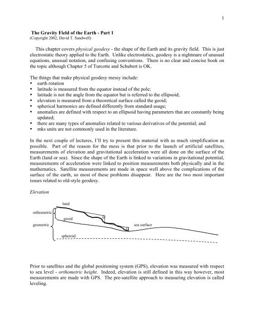
Elevation<br />
land<br />
orthometric<br />
geometric<br />
geoid<br />
sea surface<br />
spheroid<br />
Prior to satellites and <strong>the</strong> global positioning system (GPS), elevation was measured with respect<br />
to sea level - orthometric height. Indeed, elevation is still defined in this way however, most<br />
measurements are made with GPS. <strong>The</strong> pre-satellite approach to measuring elevation is called<br />
leveling.
2<br />
1. Start at sea level and call this zero elevation. (If <strong>the</strong>re were no winds, currents and tides<br />
<strong>the</strong>n <strong>the</strong> ocean surface would be an equipotential surface and all shorelines would be at<br />
exactly <strong>the</strong> same potential.)<br />
2. Sight a line inland perpendicular to a plumb line. Note that this plumb line will be<br />
perpendicular to <strong>the</strong> equipotential surface and thus is not pointed toward <strong>the</strong> geocenter.<br />
3. Measure <strong>the</strong> height difference and <strong>the</strong>n move <strong>the</strong> setup inland and to repeat <strong>the</strong><br />
measurements until you reach <strong>the</strong> next shoreline. If all measurements are correct you will<br />
be back to zero elevation assuming <strong>the</strong> ocean surface is an equipotential surface.<br />
After artificial satellites measuring geometric height is easier, especially if one is far from a<br />
coastline.<br />
1. Calculate <strong>the</strong> x,y,z position <strong>of</strong> each GPS satellite in <strong>the</strong> constellation using a global tracking<br />
network.<br />
2. Measure <strong>the</strong> travel time to 4 or more satellites, 3 for position and one for clock error.<br />
3. Establish your x,y,z position and convert this to height above <strong>the</strong> spheroid which we’ll<br />
define below.<br />
4. Go to a table <strong>of</strong> geoid height and subtract <strong>the</strong> local geoid height to get <strong>the</strong> orthometric height<br />
used by all surveyors and mappers.<br />
Orthometric heights are useful because water flows downhill in this system while it does not<br />
always flow downhill in <strong>the</strong> geometric height system. Of course <strong>the</strong> problem with orthometric<br />
heights is that <strong>the</strong>y are very difficult to measure or one must have a precise measurement <strong>of</strong><br />
geoid height. Let geodesists worry about <strong>the</strong>se issues.<br />
<strong>Gravity</strong><br />
<strong>The</strong> second complication in <strong>the</strong> pre-satellite geodesy is <strong>the</strong> measurement <strong>of</strong> gravity.<br />
Interpretation <strong>of</strong> surface gravity measurement is ei<strong>the</strong>r difficult or trivial depending whe<strong>the</strong>r you<br />
are on land or at sea, respectively. Consider <strong>the</strong> land case illustrated below.<br />
would like to know gravity on this surface<br />
land<br />
observations<br />
geoid<br />
Small variations in <strong>the</strong> acceleration <strong>of</strong> gravity (< 10 -6 g) can be measured on <strong>the</strong> land surface.<br />
<strong>The</strong> major problem is that when <strong>the</strong> measurement is made in a valley, <strong>the</strong>re are masses above <strong>the</strong><br />
observation plane. Thus, bringing <strong>the</strong> gravity measurement to a common level requires
3<br />
knowledge <strong>of</strong> <strong>the</strong> mass distribution above <strong>the</strong> observation point. <strong>This</strong> requires knowledge <strong>of</strong><br />
both <strong>the</strong> geometric topography and <strong>the</strong> 3-D density. We could assume a constant density and use<br />
leveling to get <strong>the</strong> orthometric height but we need to convert to geometric height to do <strong>the</strong><br />
gravity correction. To calculate <strong>the</strong> geometric height we need to know <strong>the</strong> geoid but <strong>the</strong> geoid<br />
height measurement comes from <strong>the</strong> gravity measurement so <strong>the</strong>re is no exact solution. Of<br />
course one can make some approximations to get around this dilemma but it is still a problem<br />
and this is <strong>the</strong> fundamental reason why many geodesy books are so complicated. Of course if<br />
one could make measurements <strong>of</strong> both <strong>the</strong> gravity and topography on a plane (or sphere) above<br />
all <strong>of</strong> <strong>the</strong> topography, our troubles would be over.<br />
Ocean gravity measurements are much less <strong>of</strong> a problem because <strong>the</strong> ocean surface is nearly<br />
equal to <strong>the</strong> geoid so we can simply define <strong>the</strong> ocean gravity measurement as free-air gravity.<br />
We’ll get back to all <strong>of</strong> this again later when we discuss flat-earth approximations for gravity<br />
analysis.<br />
GLOBAL GRAVITY (References: Turcotte and Schubert Geodynamics, Ch. 5. p. 198-212; Stacey, Physics <strong>of</strong><br />
<strong>the</strong> <strong>Earth</strong>, Ch. 2+3; Jackson, Electrodynamics, Ch. 3; Fowler, <strong>The</strong> Solid <strong>Earth</strong>, Ch. 5.)<br />
<strong>The</strong> gravity field <strong>of</strong> <strong>the</strong> <strong>Earth</strong> can be decomposed as follows:<br />
• <strong>the</strong> main field due to <strong>the</strong> total mass <strong>of</strong> <strong>the</strong> earth;<br />
• <strong>the</strong> second harmonic due to <strong>the</strong> flattening <strong>of</strong> <strong>the</strong> <strong>Earth</strong> by rotation; and<br />
• anomalies which can be expanded in spherical harmonics or fourier series.<br />
<strong>The</strong> combined main field and <strong>the</strong> second harmonic make up <strong>the</strong> reference earth model (i.e.,<br />
spheroid, <strong>the</strong> reference potential, and <strong>the</strong> reference gravity). Deviations from this reference<br />
model are called elevation, geoid height, deflections <strong>of</strong> <strong>the</strong> vertical, and gravity anomalies.<br />
Spherical <strong>Earth</strong> Model<br />
<strong>The</strong> spherical earth model is a good point to define some <strong>of</strong> <strong>the</strong> unusual geodetic terms. <strong>The</strong>re<br />
are both fundamental constants and derived quantities.<br />
parameter description formula value/unit<br />
R e mean radius <strong>of</strong> earth - 6371000 m<br />
M e mass <strong>of</strong> earth - 5.98 x 10 24 kg<br />
G gravitational constant - 6.67x10 –11 m 3 kg –1 s –2<br />
ρ mean density <strong>of</strong> earth M e (4/3π R 3 e ) -1 5520 kg m –3<br />
U mean potential energy -GM e R -1 e -6. 26x10 -7 m 2 s –2<br />
needed to take a unit<br />
mass from <strong>the</strong> surface<br />
<strong>of</strong> <strong>the</strong> earth and place<br />
it at infinite distance<br />
g mean acceleration on<br />
<strong>the</strong> surface <strong>of</strong> <strong>the</strong><br />
earth<br />
-δU/δr = -GM e R -2 e -9.82 m s –2<br />
δg/δr<br />
gravity gradient or<br />
free-air correction<br />
δg/δr = -2GM e R e –3<br />
= -2g/R e<br />
3.086 x10 -6 s –2
4<br />
We should say a little more about units. Deviations in acceleration from <strong>the</strong> reference model,<br />
described next, are measured in units <strong>of</strong> milligal (1 mgal = 10 -3 cm s -2 =10 -5 m s –2 = 10 gravity<br />
units (gu)). As notes above <strong>the</strong> vertical gravity gradient is also called <strong>the</strong> free-air correction<br />
since it is <strong>the</strong> first term in <strong>the</strong> Taylor series expansion for gravity about <strong>the</strong> radius <strong>of</strong> <strong>the</strong> earth.<br />
∂g<br />
gr ( ) = gR (<br />
r r R<br />
e) + ( −<br />
e)+<br />
....<br />
∂<br />
(1)<br />
Example: How does one measure <strong>the</strong> mass <strong>of</strong> <strong>the</strong> <strong>Earth</strong> <strong>The</strong> best method is to time <strong>the</strong> orbital<br />
period <strong>of</strong> an artificial satellite. Indeed measurements <strong>of</strong> all long-wavelength gravitational<br />
deviations from <strong>the</strong> reference model are best done be satellites.<br />
GMe<br />
r<br />
m<br />
v<br />
GMem<br />
2<br />
r<br />
=<br />
mv<br />
r<br />
2<br />
(2)<br />
GM<br />
2<br />
r<br />
e<br />
= rω<br />
⇒ GM = r ω<br />
2 3 2<br />
s e s<br />
<strong>The</strong> mass is in orbit about <strong>the</strong> center <strong>of</strong> <strong>the</strong> <strong>Earth</strong> so <strong>the</strong> outward centrifugal force is balanced by<br />
<strong>the</strong> inward gravitational force; this is Kepler’s third law. If we measure <strong>the</strong> radius <strong>of</strong> <strong>the</strong> satellite<br />
orbit r and <strong>the</strong> orbital frequency ω s , we can estimate GM e . For example <strong>the</strong> satellite Geosat has<br />
a orbital radius <strong>of</strong> 7168 km and a period <strong>of</strong> 6037.55 sec so GM e is 3.988708x10 14 m 3 s –2 . Note<br />
that <strong>the</strong> product GM e is tightly constrained by <strong>the</strong> observations but that <strong>the</strong> accuracy <strong>of</strong> <strong>the</strong> mass<br />
<strong>of</strong> <strong>the</strong> earth M e is related to <strong>the</strong> accuracy <strong>of</strong> <strong>the</strong> measurement <strong>of</strong> G.<br />
Ellipsoidal <strong>Earth</strong> Model<br />
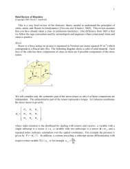
<strong>The</strong> centrifugal effect <strong>of</strong> <strong>the</strong> earth's rotation causes an equatorial bulge that is <strong>the</strong> principal<br />
departure <strong>of</strong> <strong>the</strong> earth from a spherical shape. If <strong>the</strong> earth behaved like a fluid and <strong>the</strong>re were no<br />
convective fluid motions, <strong>the</strong>n it would be in hydrostatic equilibrium and <strong>the</strong> earth would assume<br />
<strong>the</strong> shape <strong>of</strong> an ellipsoid <strong>of</strong> revolution also called <strong>the</strong> spheroid.
5<br />
c<br />
a<br />
θ<br />
θ g<br />
parameter description formula value/unit (WGS84)<br />
GM e 3.986004418 x 10 14 m 3 s –2<br />
a equatorial radius - 6378137 m<br />
c polar radius - 6356752.3 m<br />
ω rotation rate - 7.292115 x 10 -5 rad s -1<br />
f flattening f = (a - c)/a 1/298.257223560<br />
θ g geographic latitude - -<br />
θ geocentric latitude - -<br />
<strong>The</strong> formula for an ellipse in Cartesian co-ordinates is<br />
x<br />
a<br />
2<br />
2<br />
2 2<br />
y z<br />
+ + = 1<br />
(3)<br />
2 2<br />
a c<br />
where <strong>the</strong> x-axis is in <strong>the</strong> equatorial plane at zero longitude (Greenwich), <strong>the</strong> y-axis is in <strong>the</strong><br />
equatorial plane and at 90˚E longitude and <strong>the</strong> z-axis points along <strong>the</strong> spin-axis. <strong>The</strong> formula<br />
relating x, y, and z to geocentric latitude and longitude is<br />
x = rcosθcosφ<br />
y = rcosθsinφ<br />
z = rsinθ<br />
(4)<br />
Now we can re-write <strong>the</strong> formula for <strong>the</strong> ellipse in polar co-ordinates and solve for <strong>the</strong> radius <strong>of</strong><br />
<strong>the</strong> ellipse as a function <strong>of</strong> geocentric latitude.<br />
2 2 - 12 /<br />
⎛<br />
r = cos θ sin θ⎞<br />
2<br />
⎜ +<br />
a 1- f θ<br />
(5)<br />
2 2 ⎟ ≅ ( sin )<br />
⎝ a c ⎠
6<br />
Before satellites were available for geodetic work, one would establish latitude by measuring <strong>the</strong><br />
angle between a local plumb line and an external reference point such as Polaris. Since <strong>the</strong> local<br />
plumb line is perpendicular to <strong>the</strong> spheroid (i.e., local flattened surface <strong>of</strong> <strong>the</strong> earth), it points to<br />
one <strong>of</strong> <strong>the</strong> foci <strong>of</strong> <strong>the</strong> ellipse. <strong>The</strong> conversion between geocentric and geographic latitude is<br />
straightforward and its derivation is left as an exercise. <strong>The</strong> formulas are<br />
2<br />
c<br />
2<br />
tanθ = tanθg<br />
or tanθ = ( 1 − f ) tanθ<br />
2<br />
g<br />
(6)<br />
a<br />
(Example: What is <strong>the</strong> geocentric latitude at a geographic latitude <strong>of</strong> 45˚. <strong>The</strong> answer is θ =<br />
44.8˚ which amounts to a 22 km difference in location!)<br />
Flattening <strong>of</strong> <strong>the</strong> <strong>Earth</strong> by Rotation<br />
Suppose <strong>the</strong> earth is a rotating, self gravitating ball <strong>of</strong> fluid in hydrostatic equilibrium. <strong>The</strong>n<br />
density will increase with increasing depth and surfaces <strong>of</strong> constant pressure and density will<br />
coincide. <strong>The</strong> surface <strong>of</strong> <strong>the</strong> earth will be one <strong>of</strong> <strong>the</strong>se equipotential surfaces and it has a<br />
potential U o .<br />
U = V ( o<br />
r , θ) − 1<br />
ω 2 2<br />
r<br />
2<br />
cos 2<br />
θ<br />
(7)<br />
where <strong>the</strong> second term on <strong>the</strong> right side <strong>of</strong> equation (7) is <strong>the</strong> change potential due to <strong>the</strong> rotation<br />
<strong>of</strong> <strong>the</strong> earth at a frequency ω. <strong>The</strong> potential due to an ellipsoidal earth in a non-rotating frame<br />
can be expressed as<br />
GM<br />
V<br />
J a 2<br />
⎡<br />
e<br />
r r P J a<br />
=− − −<br />
⎛ ⎞<br />
⎤<br />
⎢1 1 1( θ) 2<br />
P2<br />
( θ ) − .......<br />
⎣<br />
⎝ r ⎠<br />
⎥<br />
(9)<br />
⎦<br />
<strong>The</strong> center <strong>of</strong> <strong>the</strong> co-ordinate system is selected to coincide with <strong>the</strong> center <strong>of</strong> mass so, by<br />
definition, J 1 is zero. For this model, we keep only J 2 (dynamic form factor or "jay two" = 1.08<br />
x 10 -3 ) so <strong>the</strong> final reference model is<br />
2<br />
GMe<br />
GMeJ2a<br />
V =− + ( 3sin 2 θ −1<br />
3<br />
)<br />
(10)<br />
r 2r<br />
<strong>This</strong> parameter J 2 is related to <strong>the</strong> principal moments <strong>of</strong> inertia <strong>of</strong> <strong>the</strong> earth by MacCullagh's<br />
formula. For a complete derivation see Stacey, p. 23-35. Let C and A be <strong>the</strong> moments <strong>of</strong><br />
intertia about <strong>the</strong> spin axis and equatorial axis respectively. For example
7<br />
C = ∫ ( 2 2<br />
x + y ) dm<br />
V<br />
After a lot <strong>of</strong> algebra one can derive a relationship between J 2 and <strong>the</strong> moments <strong>of</strong> inertia.<br />
(11)<br />
J<br />
C-<br />
A<br />
=<br />
Ma<br />
2 2<br />
(12)<br />
In addition, if we know J 2 , we can determine <strong>the</strong> flattening. <strong>This</strong> is done by inserting equation<br />
(10) into equation (7) and noting that <strong>the</strong> value <strong>of</strong> U o is <strong>the</strong> same at <strong>the</strong> equator and <strong>the</strong> pole.<br />
Solving for <strong>the</strong> polar and equatorial radaii that meet this constraint, one finds a relationship<br />
between J 2 and <strong>the</strong> flattening.<br />
f<br />
a c a<br />
= − 3 2<br />
3 1 ω<br />
= J2<br />
+<br />
(13)<br />
a 2 2 GM<br />
Thus if we could somehow measure J 2 , we would know quite a bit about our planet.<br />
Measurement <strong>of</strong> J 2<br />
Just as in <strong>the</strong> case <strong>of</strong> measuring <strong>the</strong> total mass <strong>of</strong> <strong>the</strong> earth, <strong>the</strong> best way to measure, is to<br />
monitor <strong>the</strong> orbit <strong>of</strong> an artificial satellite. In this case we measure <strong>the</strong> precessional period <strong>of</strong> <strong>the</strong><br />
inclined orbit plane. To second degree, external potential is<br />
2<br />
GMe<br />
GMeJ2a<br />
V =− + ( 3sin 2 θ −1)<br />
(14)<br />
3<br />
r 2r<br />
<strong>The</strong> force acting on <strong>the</strong> satellite is -∇V.<br />
∂V<br />
∂<br />
g =− − −<br />
∂ ∂θ θ ∂<br />
r r 1 V<br />
V<br />
ˆ ˆ 1 ˆ<br />
r r cosθ<br />
∂φ φ<br />
(15)<br />
If we were out in space, <strong>the</strong> best way to measure J 2 would be to measure <strong>the</strong> θ-component <strong>of</strong> <strong>the</strong><br />
gravity force.<br />
g<br />
θ<br />
∂V<br />
GMea J<br />
= 1 3 2<br />
2<br />
= - sinθcos θ<br />
(16)<br />
4<br />
r ∂θ r<br />
<strong>This</strong> component <strong>of</strong> force will apply a torque to <strong>the</strong> orbital angular momentum and it should be<br />
averaged over <strong>the</strong> orbit. Consider <strong>the</strong> diagram below.
8<br />
∆L<br />
L<br />
m<br />
-g θ<br />
i<br />
For a prograde orbit, <strong>the</strong> precession ω p is retrograde; that it is opposite to <strong>the</strong> earth's spin<br />
direction. <strong>The</strong> complete derivation is found in Stacey [1977, p. 76] and <strong>the</strong> result is<br />
ω<br />
ω<br />
p<br />
s<br />
a<br />
= −3 2<br />
J i<br />
2 2<br />
cos (17)<br />
2r<br />
where i is <strong>the</strong> inclination <strong>of</strong> <strong>the</strong> satellite orbit with respect to <strong>the</strong> equatorial plane, ω s is <strong>the</strong> orbit<br />
frequency <strong>of</strong> <strong>the</strong> satellite and ω p is <strong>the</strong> precession frequency <strong>of</strong> <strong>the</strong> orbit plane in inertial space.<br />
Example - LAGEOS<br />
As an example, <strong>the</strong> LAGEOS satellite orbits <strong>the</strong> earth every 13673.4 seconds at an average<br />
radius <strong>of</strong> 12,265 km, and an inclination <strong>of</strong> 109.8˚. Given <strong>the</strong> parameters in <strong>the</strong> table above and<br />
J 2 = 1.08 x 10 -3 , <strong>the</strong> predicted precession rate is 0.337˚/day. <strong>This</strong> can be compared with <strong>the</strong><br />
observed rate <strong>of</strong> 0.343˚/day. <strong>The</strong> figure on <strong>the</strong> next page is an illustration <strong>of</strong> <strong>the</strong> LAGEOS<br />
satellite.<br />
Hydrostatic Flattening<br />
Given <strong>the</strong> radial density structure, <strong>the</strong> earth rotation rate and <strong>the</strong> assumption <strong>of</strong> hydrostatic<br />
equilibrium, one can calculate <strong>the</strong> <strong>the</strong>oretical flattening <strong>of</strong> <strong>the</strong> earth (see Garland, <strong>The</strong> <strong>Earth</strong>'s<br />
Shape and <strong>Gravity</strong>, Permagon, 1977, Appendix 2). <strong>This</strong> is called <strong>the</strong> hydrostatic flattening f h =<br />
1/299.5. From <strong>the</strong> table above we have <strong>the</strong> observed flattening f = 1/298.257 so <strong>the</strong> actual earth<br />
is flatter than <strong>the</strong> <strong>the</strong>oretical earth. <strong>The</strong>re are two reasons for this. First, <strong>the</strong> earth is still<br />
recovering from <strong>the</strong> last ice age when <strong>the</strong> poles were loaded by heavy ice sheets. When <strong>the</strong> ice<br />
melted polar dimples remained and <strong>the</strong> glacial rebound <strong>of</strong> <strong>the</strong> viscous mantle is still incomplete.<br />
Second, <strong>the</strong> mantle is not in hydrostatic equilibrium because <strong>of</strong> mantle convection. Finally it<br />
should be noted that J 2 is changing with time due to <strong>the</strong> continual post-glacial rebound. <strong>This</strong> is<br />
called "jay two dot" and it can be observed in satellite orbits as a time variation in <strong>the</strong> precession<br />
rate.