Lecture 11: Passive Microwave Remote Sensing

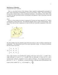
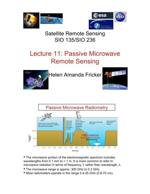
Satellite Remote SensingSIO 135/SIO 236Lecture 11: Passive MicrowaveRemote SensingHelen Amanda FrickerPassive Microwave Radiometrymicrowave•! The microwave portion of the electromagnetic spectrum includeswavelengths from 0.1 mm to > 1 m. It is more common to refer tomicrowave radiation in terms of frequency, f, rather than wavelength, !.•! The microwave range is approx. 300 GHz to 0.3 GHz.•! Most radiometers operate in the range 0.4-35 GHz (0.8-75 cm).

Microwave Brightness Temperature•! Microwave radiometers can measure the emittedspectral radiance received (L ! ) "•! This is called the brightness temperature and islinearly related to the kinetic temperature of thesurface•! The Rayleigh-Jeans approximation provides a simplelinear relationship between measured spectralradiance temperature and emissivityAt the long wavelengths,of the microwave region,the relationship betweenspectral emittance andwavelength can beapproximated by astraight line.!

Microwave Brightness Temperature!T is also called the “brightnesstemperature” typically shown as T BT B= !42kc L !Microwave Brightness Temperature•! Brightness temperature can be related to kinetictemperature through the emissivity of the material, i.e. itsability to emit radiation.T b= !T kin•! So passive microwave brightness temperatures can beused to monitor temperature as well as properties related toemissivity•! In the microwave region, materials have large variations inemissivity

Passive Microwave Applications•! Soil moisture•! Snow water equivalent•! Sea-ice extent, concentration and type (and lake ice)•! Sea surface temperature•! Atmospheric water vapor•! Surface wind speed only over the oceans!•! Cloud liquid water•! Rainfall rateMonitoring Temperatures with Passive Microwave•! Sea surfacetemperature•! Land surfacetemperature

Passive Microwave Remote Sensing from SpaceAdvantages•! Penetration through nonprecipitatingclouds•! Radiance is linearly relatedto temperature (i.e. theretrieval is nearly linear)•! Highly stable instrumentcalibration•! Global coverage and wideswathDisadvantages•! Larger field of views(10-50 km) compared toVIS/IR sensors•! Variable emissivity overland•! Polar orbiting satellitesprovide discontinuoustemporal coverage atlow latitudes (need tocreate weeklycomposites)Sea-ice•! Sea ice is frozen seawater floating on the ocean surface•! Sea-ice has an insulating effect on the ocean (traps heat) &affects the Earth’s albedo•! Some sea ice is semi-permanent, persisting from year to year,and some is seasonal, melting and refreezing from season toseason.•! The sea ice cover reaches its minimum extent at the end ofeach summer and the remaining ice is called the perennial icecover.•! Passive microwave data have shown that the spatial extent ofthe Arctic sea-ice cover is shrinking

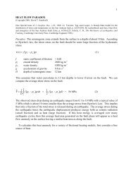
Passive Microwave Remote Sensing from SpaceMeasures thermal emissions - as for Thermal IR, but atlonger wavelengths."Rayleigh-Jeans approximation:"T B = T s # (!, $)"Large contrast in # of open ocean (~0.4 @18 GHz) & sea ice "" " " " " "(~0.9 @ 18 GHz)"Sea Ice Extent"Combine 19 & 37GHz data "Sea Ice Concentration"Emissivities of sea-ice types and open water atmicrowave frequenciesMassom (in press) after Svendsen et al. (1993)

Sea-ice monitoringSuppose we measure the thermal emissions at 10 GHz in a polarocean which has a mixture of open seawater, young sea ice, and oldsea ice. It is a warm day so both the ice and water are at the meltingpoint.At 10 GHz (~3 cm), the EMR waves penetrate ~1 mm into theseawater and ~1 m into the ice.Emissivities: seawater = 0.4young ice = 0.95old ice = 0.85T bBrightness temperature observed by the radiometer aboard thespacecraft will reflect the variations in the emissivity of the surface.This is an excellent way to monitor the ice cover of the polar oceansand discriminate first-year ice from multi-year ice. "The Passive Microwave Radiometer is the “Bread and Butter” Sensorfor Measuring Sea-Ice Concentration and ExtentDMSP SSM/IMonthly Means~3 million km 2 ! ~19 million km 2 !In Operation Since 1973Poor Spatial Resolution (25km)But Penetrates Cloud and Darkness, + Complete Daily Coverage

Summer 2007: A new record lowStroeve et al. 2008"Sea-ice monitoringPredictions for the future

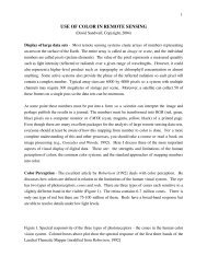
Satellite Remote SensingSIO 135/SIO 236Lecture 12: Satellite Radar and LaserAltimetryHelen Amanda FrickerERS-1 operating principlesSatellite!!Rc!transmittedpulseTreturnedpulse•! Altimeter measures the time delay (T) taken for a radar pulse to travel to thesurface and back again•! Range (R) from the satellite to the surface is determined from the time delayfrom the equation R = cT/2 where c is the propagation velocity of e/m waves infree space

Radar altimeter height measurementIf satellite altitude (A) known, surface height (h) can be determined from range (R)h ( $ ,#,t ) = "( $ ,#,t ) ! R($ ,#,t )

&-parameter retracking (GSFC)Range windowReturnpower(counts)Nine parameter fit (& 1 -& 9 )2 nd retracking point! 8 (2 nd trailingedge slope)! 9 (1 st trailingedge slope)! 7 (2 nd risetime)! 6! 4 (1 st risetime)! 71 st retracking point! 1! 3! 20 31 63Range bin number•! Used for 'complex' waveforms, with two leading edges - occurs when twomain reflecting surfaces at different ranges contribute to return power•! Two parameters (# 3& # 6) define leading edges, providing two correctionsOffset Center of Gravity (OCOG) retrackerReturnpower(counts)Range windowT 50%Amplitude = 2 x amplitudeof COG of waveformA = 2!!0.5 ppn2nIn practice, square ofwaveform power (p n2)used to calculate AT 25%T 10%0 31 63Range bin number•! Waveform amplitude (A) determined•! Threshold value, T x%, is pre-defined % of A - 1st bin on leading edge with valueexceeding T x%determined. Linear interpolation between this bin & precedingbin provides location of retrack point on leading edge [x = 10, 25 or 50%]AA64!5=64!5pp4n2n

Effect of slope and roughness on laseraltimeter waveforms•! Returned pulse broadened by thedistribution of surface heights in thefootprint•! Return waveform is convolution oftransmitted pulse with heightdistribution function•! Knowledge of transmitted pulse iscritical - can retrieve throughdeconvolution if roll angle is largeICESat laser altimeterALTIMETER!Geoscience Laser Altimeter System (GLAS) " ! Measures distance to ice,land, water, or clouds fromlaser pulse "time of flight" (d= r x t)" ! Digitizes the transmittedand received 1064-nm pulsewaveforms" ! Laser-beam attitude fromstar-trackers and internalangle systemSchematic of single profile science datameasurements, compiled through time tobuild elevation data sets!ATMOSPHERIC LIDAR!" ! Measures laser backscatteringfrom clouds andaerosols" ! Data from 532 nm and 1064nm pulses" ! Photon counting/along-tracksignal integration" ! Simultaneous operationwith altimeter

Effect of slope and roughnesson " ICESat ! Returned waveformspulse broadened by thedistribution of surface heights inthe footprint" ! Return waveform is convolution oftransmitted pulse with heightdistribution function" ! Knowledge of transmitted pulse iscritical - can retrieve throughdeconvolution if roll angle is largeICESat range measurement•! Output pulserecorded•! 32 gates•! pulse width 4ns•! Digitised in 1ns (15cm)range bins•! 544 range bins recordedover ice & 200 over ocean•! Range measurement derived from travel timeof laser pulse, using waveform centroid asreference point•! Centroid valid over most ice surfaces wheresingle Gauss fit is appropriate, but not fordouble peaked waveforms resulting from twosurfaces in footprint

Satellite Remote SensingSIO 135/SIO 236Lecture 13: Applications of satellitealtimetry over iceHelen Amanda FrickerIce shelf grounding zone (GZ)Tide model of Ross Ice Shelf run over 25hours" !Transition zone between fullyfloating & fully grounded ice" !Often poorly defined by pre-ICESat datasets" !Regions of significant basal melt" !Complex physics: coupling ofbedrock, till, ice & ocean" !Can rapidly evolve in response tochanges in ice thickness & sealevel" !Monitoring GZs is important part ofice sheet change detection, theprimary goal of the ICESat Mission

Features near the grounding zone!H: inshore limit of the hydrostatic zone of free floating ice shelf iceI: inflexion point - in some cases this may just be a change in slopeG: limit of ice flotationF: limit of ice flexure from tidal movementRelative locations of these features will change depending on ice thickness, bedrocktopography & properties etc.FGIHice shelftidal motionof floatingshelfbedrockoceanadapted from Vaughan, 1994Repeat track data filtering usinggain and return energyGAINValues of gain above ~50 andenergies below ~10fJ areindicators of cloudsENERGYTide predictions fromCATS02.01ICESat elevations (top) & anomalies(bottom) for all 7 operations periodsGain & energy for all repeats: notehigh gain and low energy for Laser2c & Laser 3d

Repeat track data filtering usinggain and return energyInflexion pointGAINValues of gain above ~50 andenergies below ~10fJ areindicators of cloudsGZ width ~9km along-trackENERGYLimit of flexureSeaward GZ limitGain & energy for all repeats: notehigh gain and low energy for Laser2c & Laser 3dThe effect of clouds!! On Kamb Ice Stream:this signal looked justlike a water event…but……it wasn’t!

Examples of some “real” eventsFricker & Padman(GRL, 2006)Tide-induced flexure•!•!•!•!Events located in topographic basinsNo lateral variations in anomaly extent during growth or decayAnomalies showed clear flexural boundariesChanges had short time scalesSatellite image differencingElevation range 2003-06 (m)ConwayRidgeEngelhardtRidge0 9mUplift" ! Two of the largest regions: sign ofchange confirmed by image differencing" ! Combined several MODIS images fromNovember and December each year togenerate one data cumulation image forthat year" ! Differencing these images -- subtractingthe pixel values -- emphasizes areaswhere surface slope changedMOA (NSIDC)Subsidence+ indicates surface uplift (filling)-! indicates surface deflation (draining)~ indicates oscillating (i.e. doing both)

New subglacial lake inventory1.0Volume range (km 3 )0.1Active lakes from ICESat 2003-07123 lakes totalSiegert/Wingham/Bell lakesEarth Section seminar - April 28 20080.01Ben Smith et al. in prep