Meshfree and particle methods and their applications - TAM ...
Meshfree and particle methods and their applications - TAM ...
Meshfree and particle methods and their applications - TAM ...

Create successful ePaper yourself
Turn your PDF publications into a flip-book with our unique Google optimized e-Paper software.
6 Li <strong>and</strong> Liu: <strong>Meshfree</strong> <strong>and</strong> <strong>particle</strong> <strong>methods</strong> <strong>and</strong> <strong>applications</strong> Appl Mech Rev vol 55, no 1, January 2002<br />
Monte Carlo estimates of integral interpolants. The error of<br />
r<strong>and</strong>om interpolation was first estimated by Niedereiter 162<br />
as being N 1 log N n1 where N is total <strong>particle</strong> number <strong>and</strong><br />
n is the dimension of space. This result was further improved<br />
by Wozniakowski 163 as being N 1 log N n1/2 . According<br />
to reference 104, ‘‘this remarkable result was produced<br />
by a challenge with a payoff of sixty-four dollars !’’ Twentyone<br />
years after its invention, in 1998 Di Lisio et al 164<br />
gave a convergence proof of smoothed <strong>particle</strong> hydrodynamics<br />
method for regularized Euler flow equations.<br />
Besides consistency conditions, the conservation properties<br />
of a SPH formulation also strongly influence its performance.<br />
This has been a critical theme throughout SPH research,<br />
see 12,104,120,145,155,165. It is well known that<br />
classical SPH enjoys Galilean invariance, <strong>and</strong> if certain derivative<br />
approximations, or Golden rules as Monaghan puts<br />
it, are chosen, the corresponding SPH formulations can preserve<br />
some discrete conservation laws. This issue was recently<br />
revisited by Bonet et al 166, <strong>and</strong> they set forth a<br />
discrete variational SPH formulation, which can automatically<br />
satisfy the balance of linear momentum <strong>and</strong> balance of<br />
angular momentum conservation laws. Here is the basic idea.<br />
Assume the discrete potential energy in a SPH system is<br />
x<br />
I<br />
V I 0 UJ I (18)<br />
where V I 0 is the initial volume element, <strong>and</strong> U(J I ) is the<br />
internal energy density, which is assumed to be the function<br />
of determinant of the Jacobian—ratio between the initial <strong>and</strong><br />
current volume element,<br />
J V I<br />
V I<br />
0 I 0<br />
I<br />
(19)<br />
where I 0 <strong>and</strong> I are pointwise density in initial configuration<br />
<strong>and</strong> in current configuration.<br />
For adiabatic processes, the pressure can be obtained from<br />
U I /J p I . Thus, the stationary condition of potential energy<br />
gives<br />
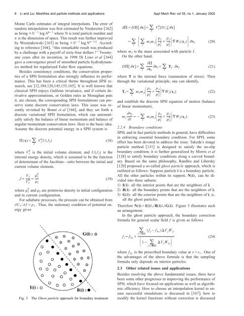
Fig. 3<br />
The Ghost <strong>particle</strong> approach for boundary treatment<br />
Dv V 0 I DU I v<br />
I<br />
<br />
I<br />
m I m<br />
J<br />
J p I<br />
2 p J<br />
I J<br />
2 W I x J v I (20)<br />
where m I is the mass associated with <strong>particle</strong> I.<br />
On the other h<strong>and</strong>,<br />
<br />
Dv v<br />
I x I<br />
I<br />
T I •v I (21)<br />
I<br />
where T is the internal force summation of stress. Then<br />
through the variational principle, one can identify,<br />
T I m I m<br />
I<br />
J p I<br />
2 p J<br />
I J<br />
2 W I x J (22)<br />
<strong>and</strong> establish the discrete SPH equation of motion balance<br />
of linear momentum,<br />
dv I<br />
m I<br />
dt m I m<br />
I<br />
J p I<br />
2 p J<br />
W<br />
I x J . (23)<br />
I<br />
2.2.4 Boundary conditions<br />
SPH, <strong>and</strong> in fact <strong>particle</strong> <strong>methods</strong> in general, have difficulties<br />
in enforcing essential boundary condition. For SPH, some<br />
effort has been devoted to address the issue. Takeda’s image<br />
<strong>particle</strong> method 131 is designed to satisfy the no-slip<br />
boundary condition; it is further generalized by Morris et al<br />
128 to satisfy boundary conditions along a curved boundary.<br />
Based on the same philosophy, R<strong>and</strong>les <strong>and</strong> Libersky<br />
120 proposed a so-called ghost <strong>particle</strong> approach, which is<br />
outlined as follows: Suppose <strong>particle</strong> i is a boundary <strong>particle</strong>.<br />
All the other <strong>particle</strong>s within its support, N(i), can be divided<br />
into three subsets:<br />
1 I(i): all the interior points that are the neighbors of i;<br />
2 B(i): all the boundary points that are the neighbors of i;<br />
3 G(i): all the exterior points that are the neighbors of i, ie,<br />
all the ghost <strong>particle</strong>s.<br />
Therefore N(i)I(i)B(i)G(i). Figure 3 illustrates such<br />
an arrangement.<br />
In the ghost <strong>particle</strong> approach, the boundary correction<br />
formula for general scalar field f is given as follows<br />
f i f bc <br />
J<br />
2<br />
f j f bc V j W ij<br />
jI„i…<br />
1<br />
jB„i…<br />
V j W ij<br />
(24)<br />
where f bc is the prescribed boundary value at xx i . One of<br />
the advantages of the above formula is that the sampling<br />
formula only depends on interior <strong>particle</strong>s.<br />
2.3 Other related issues <strong>and</strong> <strong>applications</strong><br />
Besides resolving the above fundamental issues, there have<br />
been some other progresses in improving the performance of<br />
SPH, which have focused on <strong>applications</strong> as well as algorithmic<br />
efficiency. How to choose an interpolation kernel to ensure<br />
successful simulations is discussed in 167; how to<br />
modify the kernel functions without correction is discussed