Meshfree and particle methods and their applications - TAM ...
Meshfree and particle methods and their applications - TAM ...
Meshfree and particle methods and their applications - TAM ...

You also want an ePaper? Increase the reach of your titles
YUMPU automatically turns print PDFs into web optimized ePapers that Google loves.
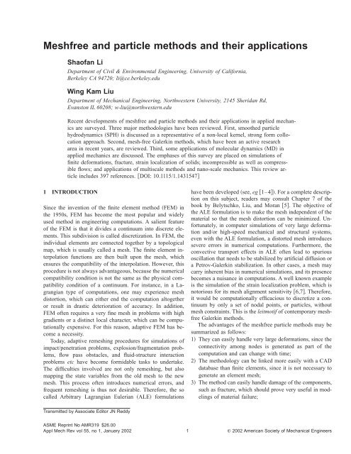
<strong>Meshfree</strong> <strong>and</strong> <strong>particle</strong> <strong>methods</strong> <strong>and</strong> <strong>their</strong> <strong>applications</strong><br />
Shaofan Li<br />
Department of Civil & Environmental Engineering, University of California,<br />
Berkeley CA 94720; li@ce.berkeley.edu<br />
Wing Kam Liu<br />
Department of Mechanical Engineering, Northwestern University, 2145 Sheridan Rd,<br />
Evanston IL 60208; w-liu@northwestern.edu<br />
Recent developments of meshfree <strong>and</strong> <strong>particle</strong> <strong>methods</strong> <strong>and</strong> <strong>their</strong> <strong>applications</strong> in applied mechanics<br />
are surveyed. Three major methodologies have been reviewed. First, smoothed <strong>particle</strong><br />
hydrodynamics SPH is discussed as a representative of a non-local kernel, strong form collocation<br />
approach. Second, mesh-free Galerkin <strong>methods</strong>, which have been an active research<br />
area in recent years, are reviewed. Third, some <strong>applications</strong> of molecular dynamics MD in<br />
applied mechanics are discussed. The emphases of this survey are placed on simulations of<br />
finite deformations, fracture, strain localization of solids; incompressible as well as compressible<br />
flows; <strong>and</strong> <strong>applications</strong> of multiscale <strong>methods</strong> <strong>and</strong> nano-scale mechanics. This review article<br />
includes 397 references. DOI: 10.1115/1.1431547<br />
1 INTRODUCTION<br />
Since the invention of the finite element method FEM in<br />
the 1950s, FEM has become the most popular <strong>and</strong> widely<br />
used method in engineering computations. A salient feature<br />
of the FEM is that it divides a continuum into discrete elements.<br />
This subdivision is called discretization. In FEM, the<br />
individual elements are connected together by a topological<br />
map, which is usually called a mesh. The finite element interpolation<br />
functions are then built upon the mesh, which<br />
ensures the compatibility of the interpolation. However, this<br />
procedure is not always advantageous, because the numerical<br />
compatibility condition is not the same as the physical compatibility<br />
condition of a continuum. For instance, in a Lagrangian<br />
type of computations, one may experience mesh<br />
distortion, which can either end the computation altogether<br />
or result in drastic deterioration of accuracy. In addition,<br />
FEM often requires a very fine mesh in problems with high<br />
gradients or a distinct local character, which can be computationally<br />
expensive. For this reason, adaptive FEM has become<br />
a necessity.<br />
Today, adaptive remeshing procedures for simulations of<br />
impact/penetration problems, explosion/fragmentation problems,<br />
flow pass obstacles, <strong>and</strong> fluid-structure interaction<br />
problems etc have become formidable tasks to undertake.<br />
The difficulties involved are not only remeshing, but also<br />
mapping the state variables from the old mesh to the new<br />
mesh. This process often introduces numerical errors, <strong>and</strong><br />
frequent remeshing is thus not desirable. Therefore, the so<br />
called Arbitrary Lagrangian Eulerian ALE formulations<br />
have been developed see, eg 1–4. For a complete description<br />
on this subject, readers may consult Chapter 7 of the<br />
book by Belytschko, Liu, <strong>and</strong> Moran 5. The objective of<br />
the ALE formulation is to make the mesh independent of the<br />
material so that the mesh distortion can be minimized. Unfortunately,<br />
in computer simulations of very large deformation<br />
<strong>and</strong>/or high-speed mechanical <strong>and</strong> structural systems,<br />
even with the ALE formulation, a distorted mesh introduces<br />
severe errors in numerical computations. Furthermore, the<br />
convective transport effects in ALE often lead to spurious<br />
oscillation that needs to be stabilized by artificial diffusion or<br />
a Petrov-Galerkin stabilization. In other cases, a mesh may<br />
carry inherent bias in numerical simulations, <strong>and</strong> its presence<br />
becomes a nuisance in computations. A well known example<br />
is the simulation of the strain localization problem, which is<br />
notorious for its mesh alignment sensitivity 6,7. Therefore,<br />
it would be computationally efficacious to discretize a continuum<br />
by only a set of nodal points, or <strong>particle</strong>s, without<br />
mesh constraints. This is the leitmotif of contemporary meshfree<br />
Galerkin <strong>methods</strong>.<br />
The advantages of the meshfree <strong>particle</strong> <strong>methods</strong> may be<br />
summarized as follows:<br />
1 They can easily h<strong>and</strong>le very large deformations, since the<br />
connectivity among nodes is generated as part of the<br />
computation <strong>and</strong> can change with time;<br />
2 The methodology can be linked more easily with a CAD<br />
database than finite elements, since it is not necessary to<br />
generate an element mesh;<br />
3 The method can easily h<strong>and</strong>le damage of the components,<br />
such as fracture, which should prove very useful in modelings<br />
of material failure;<br />
Transmitted by Associate Editor JN Reddy<br />
ASME Reprint No AMR319 $26.00<br />
Appl Mech Rev vol 55, no 1, January 2002<br />
1<br />
© 2002 American Society of Mechanical Engineers
2 Li <strong>and</strong> Liu: <strong>Meshfree</strong> <strong>and</strong> <strong>particle</strong> <strong>methods</strong> <strong>and</strong> <strong>applications</strong> Appl Mech Rev vol 55, no 1, January 2002<br />
4 Accuracy can be controlled more easily, since in areas<br />
where more refinement is needed, nodes can be added<br />
quite easily h-adaptivity;<br />
5 The continuum meshfree <strong>methods</strong> can be used to model<br />
large deformations of thin shell structures, such as nanotubes;<br />
6 The method can incorporate an enrichment of fine scale<br />
solutions of features, such as discontinuities as a function<br />
of current stress states, into the coarse scale; <strong>and</strong><br />
7 <strong>Meshfree</strong> discretization can provide accurate representation<br />
of geometric object.<br />
In general, <strong>particle</strong> <strong>methods</strong> can be classified based on<br />
two different criteria: physical principles, or computational<br />
formulations. According to the physical modeling, they may<br />
be categorized into two classes: those based on deterministic<br />
models, <strong>and</strong> those based on probabilistic models. On the<br />
other h<strong>and</strong>, according to computational modelings, they may<br />
be categorized into two different types as well: those serving<br />
as approximations of the strong forms of partial differential<br />
equations PDEs, <strong>and</strong> those serving as approximations of<br />
the weak forms of PDEs. In this survey, the classification<br />
based on computational strategies is adopted.<br />
To approximate the strong form of a PDE using a <strong>particle</strong><br />
method, the partial differential equation is usually discretized<br />
by a specific collocation technique. Examples are smoothed<br />
<strong>particle</strong> hydrodynamics SPH 8–12, the vortex method<br />
13–18, the generalized finite difference method 19,20,<br />
<strong>and</strong> many others. It is worth mentioning that some <strong>particle</strong><br />
<strong>methods</strong>, such as SPH <strong>and</strong> vortex <strong>methods</strong>, were initially<br />
developed as probabilistic <strong>methods</strong> 10,14, <strong>and</strong> it turns out<br />
that both SPH <strong>and</strong> the vortex method are most frequently<br />
used as deterministic <strong>methods</strong> today. Nevertheless, the majority<br />
of <strong>particle</strong> <strong>methods</strong> in this category are based on<br />
probabilistic principles, or used as probabilistic simulation<br />
tools. There are three major <strong>methods</strong> in this category: 1<br />
molecular dynamics both quantum molecular dynamics<br />
21–26 <strong>and</strong> classical molecular dynamics 27–32; 2 direct<br />
simulation Monte Carlo DSMC, or Monte Carlo<br />
method based molecular dynamics, such as quantum Monte<br />
Carlo <strong>methods</strong> 33–41 It is noted that not all the Monte<br />
Carlo <strong>methods</strong> are meshfree <strong>methods</strong>, for instance, a probabilistic<br />
finite element method is a mesh-based method 42–<br />
44; <strong>and</strong> 3 the lattice gas automaton LGA, or lattice gas<br />
cellular automaton 45–49 <strong>and</strong> its later derivative, the Lattice<br />
Boltzmann Equation method LBE 50–54. It may be<br />
pointed out that the Lattice Boltzmann Equation method is<br />
not a meshfree method, <strong>and</strong> it requires a grid; this example<br />
shows that <strong>particle</strong> <strong>methods</strong> are not always meshfree.<br />
The second class of <strong>particle</strong> <strong>methods</strong> is used with various<br />
Galerkin weak formulations, which are called meshfree<br />
Galerkin <strong>methods</strong>. Examples in this class are Diffuse Element<br />
Method DEM 55–58, Element Free Galerkin<br />
Method EFGM 59–63, Reproducing Kernel Particle<br />
Method RKPM 64–72, h-p Cloud Method 73–76, Partition<br />
of Unity Method 77–79, Meshless Local Petrov-<br />
Galerkin Method MLPG 80–83, Free Mesh Method 84–<br />
88, <strong>and</strong> others.<br />
There are exceptions to this classification, because some<br />
<strong>particle</strong> <strong>methods</strong> can be used in both strong form collocation<br />
as well as weak form discretization. The <strong>particle</strong>-in-cell<br />
PIC method is such an exception. The strong form collocation<br />
PIC is often called the finite-volume <strong>particle</strong>-in-cell<br />
method 89–91, <strong>and</strong> the weak form PIC is often called the<br />
material point method 92, or simply <strong>particle</strong>-in-cell method<br />
93–95. RKPM also has two versions as well: a collocation<br />
version 96 <strong>and</strong> a Galerkin weak form version 66.<br />
In areas such as astrophysics, solid state physics, biophysics,<br />
biochemistry <strong>and</strong> biomedical research, one may encounter<br />
situations where the object under consideration is not a<br />
continuum, but a set of <strong>particle</strong>s. There is no need for discretization<br />
to begin with. A <strong>particle</strong> method is the natural<br />
choice in numerical simulations. Relevant examples are the<br />
simulation of formation of a star system, the nano-scale<br />
movement of millions of atoms in a non-equilibrium state,<br />
folding <strong>and</strong> unfolding of DNA, <strong>and</strong> dynamic interactions of<br />
various molecules, etc. In fact, the current trend is not only<br />
to use <strong>particle</strong> <strong>methods</strong> as discretization tools to solve continuum<br />
problems such as SPH, vortex method 14,15,97<br />
<strong>and</strong> meshfree Galerkin <strong>methods</strong>, but also to use <strong>particle</strong><br />
<strong>methods</strong> as a physical model statistical model, or atomistic<br />
model to simulate continuum behavior of physics. The latest<br />
examples are using the Lattice Boltzmann method to solve<br />
fluid mechanics problems, <strong>and</strong> using molecular dynamics to<br />
solve fracture mechanics problems in solid mechanics 98–<br />
103.<br />
This survey is organized as follows: The first part is a<br />
critical review of smoothed <strong>particle</strong> hydrodynamics SPH.<br />
The emphasis is placed on the recent development of corrective<br />
SPH. The second part is a summary of meshfree Galerkin<br />
<strong>methods</strong>, which includes DEM, EFGM, RKPM, hp-<br />
Cloud method, partition of unity method, MLPGM, <strong>and</strong><br />
meshfree nodal integration <strong>methods</strong>. The third part reviews<br />
recent <strong>applications</strong> of molecular dynamics in fracture mechanics<br />
as well as nanomechanics. The last part is a survey<br />
on some other meshfree/<strong>particle</strong> <strong>methods</strong>, such as vortex<br />
<strong>methods</strong>, the Lattice Boltzmann method, the natural element<br />
method, the <strong>particle</strong>-in-cell method, etc. The survey is concluded<br />
with the discussions of some emerging meshfree/<br />
<strong>particle</strong> <strong>methods</strong>.<br />
2 SMOOTHED PARTICLE HYDRODYNAMICS<br />
2.1 Overview<br />
Smoothed Particle Hydrodynamics is one of the earliest <strong>particle</strong><br />
<strong>methods</strong> in computational mechanics. Early contributions<br />
have been reviewed in several articles 8,12,104. In<br />
1977, Lucy 10 <strong>and</strong> Gingold <strong>and</strong> Monaghan 9 simultaneously<br />
formulated the so-called Smoothed Particle Hydrodynamics,<br />
which is known today as SPH. Both of them were<br />
interested in the astrophysical problems, such as the formation<br />
<strong>and</strong> evolution of proto-stars or galaxies. The collective<br />
movement of those <strong>particle</strong>s is similar to the movement of a<br />
liquid, or gas flow, <strong>and</strong> it may be modeled by the governing<br />
equations of classical Newtonian hydrodynamics. Today,<br />
SPH is being used in simulations of supernovas 105, col-
Appl Mech Rev vol 55, no 1, January 2002 Li <strong>and</strong> Liu: <strong>Meshfree</strong> <strong>and</strong> <strong>particle</strong> <strong>methods</strong> <strong>and</strong> <strong>applications</strong> 3<br />
lapse as well as formation of galaxies 106–109, coalescence<br />
of black holes with neutron stars 110,111, single <strong>and</strong><br />
multiple detonations in white dwarfs 112, <strong>and</strong> even in<br />
‘‘Modeling the Universe’’ 113. Because of the distinct advantages<br />
of the <strong>particle</strong> method, soon after its debut, the SPH<br />
method was widely adopted as one of the efficient computational<br />
techniques to solve applied mechanics problems.<br />
Therefore, the term hydrodynamics really should be interpreted<br />
as mechanics in general, if the methodology is applied<br />
to other branches of mechanics rather than classical hydrodynamics.<br />
To make distinction with the classical hydrodynamics,<br />
some authors, eg Kum et al 114,115, called it<br />
Smoothed Particle Applied Mechanics.<br />
This idea of the method is somewhat contrary to the concepts<br />
of the conventional discretization <strong>methods</strong>, which discretize<br />
a continuum system into a discrete algebraic system.<br />
In astrophysical <strong>applications</strong>, the real physical system is discrete;<br />
in order to avoid singularity, a local continuous field is<br />
generated by introducing a localized kernel function, which<br />
can serve as a smoothing interpolation field. If one wishes to<br />
interpret the physical meaning of the kernel function as the<br />
probability of a <strong>particle</strong>’s position, one is dealing with a<br />
probabilistic method. Otherwise, it is only a smoothing technique.<br />
Thus, the essence of the method is to choose a smooth<br />
kernel, W(x,h) h is the smoothing length, <strong>and</strong> to use it to<br />
localize the strong form of a partial differential equation<br />
through a convoluted integration. Define SPH averaging/<br />
localization operator as<br />
A k xAx<br />
R<br />
n Wxx,hAxd x<br />
N<br />
<br />
I1<br />
Wxx I ,hAx I V I (1)<br />
One may derive a SPH discrete equation of motion from its<br />
continuous counterpart 12,116,<br />
dv<br />
dv<br />
•<br />
dt<br />
I<br />
I ⇒ I<br />
dt<br />
I<br />
The third property ensures the convergence, <strong>and</strong> the last<br />
property comes from the requirement that the smoothing kernel<br />
must be differentiable at least once. This is because the<br />
derivative of the kernel function should be continuous to<br />
prevent a large fluctuation in the force felt by the <strong>particle</strong>.<br />
The latter feature gives rise to the name smoothed <strong>particle</strong><br />
hydrodynamics.<br />
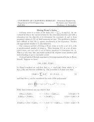
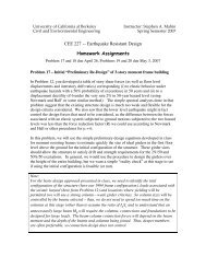
In computations, compact supported kernel functions such<br />
as spline functions are usually employed 117. In this case,<br />
the smoothing length becomes the radius of the compact support.<br />
Two examples of smooth kernel functions are depicted<br />
in Fig. 1.<br />
The advantage of using an analytical kernel is that one<br />
can evaluate a kernel function at any spatial point without<br />
knowing the local <strong>particle</strong> distribution. This is no longer true<br />
for the latest corrective smoothed <strong>particle</strong> hydrodynamics<br />
<strong>methods</strong> 66,118, because the corrective kernel function depends<br />
on the local <strong>particle</strong> distribution.<br />
The kernel representation is not only an instrument that<br />
can smoothly discretize a partial differential equation, but it<br />
also furnishes an interpolant scheme on a set of moving <strong>particle</strong>s.<br />
By utilizing this property, SPH can serve as a Lagrangian<br />
type method to solve problems in continuum mechanics.<br />
Libersky <strong>and</strong> his co-workers apply the method to<br />
solid mechanics 117,119,120, <strong>and</strong> they successfully simulate<br />
3D thick-wall bomb explosion/fragmentation problem,<br />
tungsten/plate impact/penetration problem, etc. The impact<br />
<strong>and</strong> penetration simulation has also been conducted by<br />
Johnson <strong>and</strong> his co-workers 121–123, <strong>and</strong> an SPH option<br />
is implemented in EPIC code for modeling inelastic, damage,<br />
large deformation problems. Attaway et al 124 developed<br />
a coupling technique to combine SPH with the finite<br />
element method, <strong>and</strong> an SPH option is also included in PR-<br />
ONTO 2D Taylor <strong>and</strong> Flanagan 125.<br />
SPH technology has been employed to solve problems of<br />
both compressible flow 126 <strong>and</strong> incompressible flow<br />
N<br />
<br />
J1<br />
I J •Wx I x J ,hV J (2)<br />
where is Cauchy stress, is density, v is velocity, <strong>and</strong> V J<br />
is the volume element carried by the <strong>particle</strong> J.<br />
Usually a positive function, such as the Gaussian function,<br />
is chosen as the kernel function<br />
1<br />
Wx,h <br />
h 2 n/2 exp x2<br />
h 2, 1n3 (3)<br />
where the parameter h is the smoothing length. In general,<br />
the kernel function has to satisfy the following conditions:<br />
i) Wx,h0 (4)<br />
ii) <br />
R<br />
n Wu,hd u1 (5)<br />
iii) Wu,h→u, h→0 (6)<br />
iv) Wu,hC p R n , p1 (7)<br />
Fig. 1<br />
Examples of kernel functions
4 Li <strong>and</strong> Liu: <strong>Meshfree</strong> <strong>and</strong> <strong>particle</strong> <strong>methods</strong> <strong>and</strong> <strong>applications</strong> Appl Mech Rev vol 55, no 1, January 2002<br />
116,127–129, multiple phase flow <strong>and</strong> surface tension<br />
114,115,129,130,131,132,133, heat conduction 134,<br />
electro-magnetic Maxwell equations 90,104,135, plasma/<br />
fluid motion 135, general relativistic hydrodynamics 136–<br />
138, heat conduction 134,139, <strong>and</strong> nonlinear dynamics<br />
140.<br />
2.2 Corrective SPH <strong>and</strong> other improvements<br />
in SPH formulations<br />
Various improvements of SPH have been developed through<br />
the years 104,141–149. Most of these improvement are<br />
aimed at the following shortcomings, or pathologies, in numerical<br />
computations:<br />
• tensile instability 150–154;<br />
• lack of interpolation consistency, or completeness<br />
66,155,156;<br />
• zero-energy mode 157;<br />
• difficulty in enforcing essential boundary condition<br />
120,128,131.<br />
2.2.1 Tensile instability<br />
So-called tensile instability is the situation where <strong>particle</strong>s<br />
are under a certain tensile hydrostatic stress state, <strong>and</strong> the<br />
motion of the <strong>particle</strong>s become unstable. To identify the culprit,<br />
a von Neumann stability analysis was carried out by<br />
Swegle et al 150, <strong>and</strong> by Balsara 158. Swegle <strong>and</strong> his<br />
co-workers have identified <strong>and</strong> explained the source of the<br />
tensile instability. Recently, by using von Neumann <strong>and</strong> Courant<br />
stability criterion, Belytschko et al 151 revisited the<br />
problem in the general framework of meshfree <strong>particle</strong> <strong>methods</strong>.<br />
In <strong>their</strong> analysis, finite deformation effects are also considered.<br />
Several remedies have been proposed to avoid such tensile<br />
instability. Morris proposed using special kernel functions.<br />
While successful in some cases, they do not always<br />
yield satisfactory results 152. R<strong>and</strong>les <strong>and</strong> Libersky 120<br />
proposed adding dissipative terms, which is related to conservative<br />
smoothing. Notably, Dyka et al 153,154 proposed<br />
a so-called stress point method. The essential idea of this<br />
approach is to add additional points other than SPH <strong>particle</strong>s<br />
when evaluating, or sampling, stress <strong>and</strong> other state variables.<br />
Whereas the kinematic variables such as displacement,<br />
velocity, <strong>and</strong> acceleration are still sampled at <strong>particle</strong> points.<br />
In fact, the stress point plays a similar role as the ‘‘Gauss<br />
quadrature point’’ does in the numerical integration of the<br />
Galerkin weak form. This analogy was first pointed out by<br />
Liu et al 66. This problem was revisited again recently by<br />
Chen et al 159 as well as Monaghan 148. The former<br />
proposes a special corrective smoothed-<strong>particle</strong> method<br />
CSPM to address the tensile instability problem by enforcing<br />
the higher order consistency, <strong>and</strong> the latter proposes to<br />
add an artificial force to stabilize the computation. R<strong>and</strong>les<br />
<strong>and</strong> Libersky 160 combined normalization with the usual<br />
stress point approach to achieve better stability as well as<br />
linear consistency. Apparently, the SPH tensile instability is<br />
related to the lack of consistency of the SPH interpolant. A<br />
2D stress point deployment is shown in Fig. 2.<br />
2.2.2 Zero-energy mode<br />
The zero energy mode has been discovered in both finite<br />
difference <strong>and</strong> finite element computations. A comprehensive<br />
discussion of the subject can be found in the book by Belytschko<br />
et al 5. The reason that SPH suffers similar zero<br />
energy mode deficiency is due to the fact that the derivatives<br />
of kinematic variables are evaluated at <strong>particle</strong> points by analytical<br />
differentiation rather than by differentiation of interpolants.<br />
In many cases, the kernel function reaches a maximum<br />
at its nodal position, <strong>and</strong> its spatial derivatives become<br />
zero. To avoid a zero-energy mode, or spurious stress oscillation,<br />
an efficient remedy is to adopt the stress point approach<br />
157.<br />
2.2.3 Corrective SPH<br />
As an interpolation among moving <strong>particle</strong>s, SPH is not a<br />
partition of unity, which means that SPH interpolants cannot<br />
represent rigid body motion correctly. This problem was first<br />
noticed by Liu et al 64–66. They then set forth a key notion,<br />
a correction function, which has become the central<br />
theme of the so-called corrective SPH. The idea of a corrective<br />
SPH is to construct a corrective kernel, a product of the<br />
correction function with the original kernel. By doing so, the<br />
consistency, or completeness, of the SPH interpolant can be<br />
enforced. This new interpolant is named the reproducing kernel<br />
<strong>particle</strong> method 64–66.<br />
SPH kernel functions satisfy zero-th order moment condition<br />
5. Most kernel functions satisfy higher order moment<br />
condition as well 104, for instance<br />
<br />
R<br />
xWx,hdx0. (8)<br />
These conditions only hold in the continuous form. In general<br />
they are not valid after discretization, ie<br />
NP<br />
I1<br />
Wxx I ,hx I 1 (9)<br />
NP<br />
I1<br />
xx I Wxx I ,hx I 0 (10)<br />
Fig. 2<br />
A 2D Stress point distribution<br />
where NP is the total number of the <strong>particle</strong>s. Note that condition<br />
9 is the condition of partition of unity. Since the
Appl Mech Rev vol 55, no 1, January 2002 Li <strong>and</strong> Liu: <strong>Meshfree</strong> <strong>and</strong> <strong>particle</strong> <strong>methods</strong> <strong>and</strong> <strong>applications</strong> 5<br />
kernel function can not satisfy the discrete moment conditions,<br />
a modified kernel function is introduced to enforce the<br />
discrete consistency conditions<br />
W˜ hxx I ;xC h xx I ;xWxx I ,h (11)<br />
where C h (x;xx I ) is the correction function, which can be<br />
expressed as<br />
C h x;xx I b 0 x,hb 1 x,h xx I<br />
b<br />
h 2 x,h<br />
xx I<br />
h<br />
2<br />
¯¯ (12)<br />
where b 0 (x),b 1 (x),¯ .,b n (x) are unknown functions. We<br />
can determine them to correct the original kernel function.<br />
Suppose f (x) is a sufficiently smooth function. By Taylor<br />
expansion,<br />
h<br />
f I f x I f x f x x Ix<br />
h<br />
f x<br />
2!<br />
x Ix<br />
h<br />
2<br />
h 2 ¯¯ (13)<br />
the modified kernel approximation can be written as,<br />
NP<br />
f h x<br />
I1<br />
NP<br />
<br />
I1<br />
<br />
NP<br />
<br />
I1<br />
<br />
W˜ hxx I ;xf I x I<br />
W˜ hxx I ,xx I f xh 0<br />
xx I<br />
h<br />
NP<br />
¯¯<br />
I1<br />
<br />
W˜ hxx I ,xx I f xh<br />
1 n xx I<br />
h<br />
n<br />
W˜ h<br />
xx I ,xx I f n x<br />
h n Oh n1 . (14)<br />
n!<br />
To obtain an n-th order reproducing condition, the moments<br />
of the modified kernel function must satisfy the following<br />
conditions:<br />
NP<br />
M 0 x<br />
I1<br />
NP<br />
M 1 x<br />
I1<br />
NP<br />
M n x<br />
I1<br />
W˜ hxx I ,xx I 1;<br />
xx I<br />
h<br />
W˜ hxx I ,xx I 0;<br />
xx I<br />
h<br />
<br />
n<br />
W˜ hxx I ,xx I 0;<br />
(15)<br />
Substituting the modified kernel expressions, 11 <strong>and</strong> 12<br />
into Eq. 15, we can determine the n1 coefficients, b i (x),<br />
by solving the following moment equations:<br />
m 0 x m 1 x ¯ m n x<br />
0 x,h<br />
m 1 x m 2 x ¯ m n1 x b 1 b <br />
m n x m n1 x ¯ m 2n x<br />
b n x,h<br />
0<br />
0<br />
1<br />
(16)<br />
<br />
It is worth mentioning that after introducing the correction<br />
function, the modified kernel function may not be a positive<br />
function anymore,<br />
Kxx I ” 0. (17)<br />
Within the compact support, K(xx I ) may become negative.<br />
This is the reason why Duarte <strong>and</strong> Oden refer to it as the<br />
signed partition of unity 73,74,76.<br />
There are other approaches to restoring completeness of<br />
the SPH approximation. Their emphases are not only consistency,<br />
but also on cost effectiveness. Using RKPM, or a<br />
moving-least-squares interpolant 155,156 to construct<br />
modified kernels, one has to know all the neighboring <strong>particle</strong>s<br />
that are adjacent to a spatial point where the kernel<br />
function is in evaluation. This will require an additional CPU<br />
to search, update the connectivity array, <strong>and</strong> calculate the<br />
modified kernel function pointwise. It should be noted that<br />
the calculation of the modified kernel function requires<br />
pointwise matrix inversions at each time step, since <strong>particle</strong>s<br />
are moving <strong>and</strong> the connectivity map is changing as well.<br />
Thus, using a moving least square interpolant as the kernel<br />
function may not be cost-effective, <strong>and</strong> it destroys the simplicity<br />
of SPH formulation.<br />
Several compromises have been proposed throughout the<br />
years, which are listed as follows:<br />
1 Monaghan’s symmetrization on derivative approximation<br />
104,145;<br />
2 Johnson-Beissel correction 123;<br />
3 R<strong>and</strong>les-Libersky correction 120;<br />
4 Krongauz-Belytschko correction 61;<br />
5 Chen-Beraun correction 139,140,161;<br />
6 Bonet-Kulasegaram integration correction 118;<br />
7 Aluru’s collocation RKPM 96.<br />
Since the linear reproducing condition in the interpolation is<br />
equivalent to the constant reproducing condition in the derivative<br />
of the interpolant, some of the algorithms directly<br />
correct derivatives instead of the interpolant. The Chen-<br />
Beraun correction corrects even higher order derivatives, but<br />
it may require more computational effort in multidimensions.<br />
Completeness, or consistency, closely relates to convergence.<br />
There are two types of error estimates: interpolation<br />
error <strong>and</strong> the error between exact solution <strong>and</strong> the numerical<br />
solution. The former usually dictates the latter. In conventional<br />
SPH formulations, there is no requirement for the<br />
completeness of interpolation. The <strong>particle</strong> distribution is assumed<br />
to be r<strong>and</strong>omly distributed <strong>and</strong> the summations are
6 Li <strong>and</strong> Liu: <strong>Meshfree</strong> <strong>and</strong> <strong>particle</strong> <strong>methods</strong> <strong>and</strong> <strong>applications</strong> Appl Mech Rev vol 55, no 1, January 2002<br />
Monte Carlo estimates of integral interpolants. The error of<br />
r<strong>and</strong>om interpolation was first estimated by Niedereiter 162<br />
as being N 1 log N n1 where N is total <strong>particle</strong> number <strong>and</strong><br />
n is the dimension of space. This result was further improved<br />
by Wozniakowski 163 as being N 1 log N n1/2 . According<br />
to reference 104, ‘‘this remarkable result was produced<br />
by a challenge with a payoff of sixty-four dollars !’’ Twentyone<br />
years after its invention, in 1998 Di Lisio et al 164<br />
gave a convergence proof of smoothed <strong>particle</strong> hydrodynamics<br />
method for regularized Euler flow equations.<br />
Besides consistency conditions, the conservation properties<br />
of a SPH formulation also strongly influence its performance.<br />
This has been a critical theme throughout SPH research,<br />
see 12,104,120,145,155,165. It is well known that<br />
classical SPH enjoys Galilean invariance, <strong>and</strong> if certain derivative<br />
approximations, or Golden rules as Monaghan puts<br />
it, are chosen, the corresponding SPH formulations can preserve<br />
some discrete conservation laws. This issue was recently<br />
revisited by Bonet et al 166, <strong>and</strong> they set forth a<br />
discrete variational SPH formulation, which can automatically<br />
satisfy the balance of linear momentum <strong>and</strong> balance of<br />
angular momentum conservation laws. Here is the basic idea.<br />
Assume the discrete potential energy in a SPH system is<br />
x<br />
I<br />
V I 0 UJ I (18)<br />
where V I 0 is the initial volume element, <strong>and</strong> U(J I ) is the<br />
internal energy density, which is assumed to be the function<br />
of determinant of the Jacobian—ratio between the initial <strong>and</strong><br />
current volume element,<br />
J V I<br />
V I<br />
0 I 0<br />
I<br />
(19)<br />
where I 0 <strong>and</strong> I are pointwise density in initial configuration<br />
<strong>and</strong> in current configuration.<br />
For adiabatic processes, the pressure can be obtained from<br />
U I /J p I . Thus, the stationary condition of potential energy<br />
gives<br />
Fig. 3<br />
The Ghost <strong>particle</strong> approach for boundary treatment<br />
Dv V 0 I DU I v<br />
I<br />
<br />
I<br />
m I m<br />
J<br />
J p I<br />
2 p J<br />
I J<br />
2 W I x J v I (20)<br />
where m I is the mass associated with <strong>particle</strong> I.<br />
On the other h<strong>and</strong>,<br />
<br />
Dv v<br />
I x I<br />
I<br />
T I •v I (21)<br />
I<br />
where T is the internal force summation of stress. Then<br />
through the variational principle, one can identify,<br />
T I m I m<br />
I<br />
J p I<br />
2 p J<br />
I J<br />
2 W I x J (22)<br />
<strong>and</strong> establish the discrete SPH equation of motion balance<br />
of linear momentum,<br />
dv I<br />
m I<br />
dt m I m<br />
I<br />
J p I<br />
2 p J<br />
W<br />
I x J . (23)<br />
I<br />
2.2.4 Boundary conditions<br />
SPH, <strong>and</strong> in fact <strong>particle</strong> <strong>methods</strong> in general, have difficulties<br />
in enforcing essential boundary condition. For SPH, some<br />
effort has been devoted to address the issue. Takeda’s image<br />
<strong>particle</strong> method 131 is designed to satisfy the no-slip<br />
boundary condition; it is further generalized by Morris et al<br />
128 to satisfy boundary conditions along a curved boundary.<br />
Based on the same philosophy, R<strong>and</strong>les <strong>and</strong> Libersky<br />
120 proposed a so-called ghost <strong>particle</strong> approach, which is<br />
outlined as follows: Suppose <strong>particle</strong> i is a boundary <strong>particle</strong>.<br />
All the other <strong>particle</strong>s within its support, N(i), can be divided<br />
into three subsets:<br />
1 I(i): all the interior points that are the neighbors of i;<br />
2 B(i): all the boundary points that are the neighbors of i;<br />
3 G(i): all the exterior points that are the neighbors of i, ie,<br />
all the ghost <strong>particle</strong>s.<br />
Therefore N(i)I(i)B(i)G(i). Figure 3 illustrates such<br />
an arrangement.<br />
In the ghost <strong>particle</strong> approach, the boundary correction<br />
formula for general scalar field f is given as follows<br />
f i f bc <br />
J<br />
2<br />
f j f bc V j W ij<br />
jI„i…<br />
1<br />
jB„i…<br />
V j W ij<br />
(24)<br />
where f bc is the prescribed boundary value at xx i . One of<br />
the advantages of the above formula is that the sampling<br />
formula only depends on interior <strong>particle</strong>s.<br />
2.3 Other related issues <strong>and</strong> <strong>applications</strong><br />
Besides resolving the above fundamental issues, there have<br />
been some other progresses in improving the performance of<br />
SPH, which have focused on <strong>applications</strong> as well as algorithmic<br />
efficiency. How to choose an interpolation kernel to ensure<br />
successful simulations is discussed in 167; how to<br />
modify the kernel functions without correction is discussed
Appl Mech Rev vol 55, no 1, January 2002 Li <strong>and</strong> Liu: <strong>Meshfree</strong> <strong>and</strong> <strong>particle</strong> <strong>methods</strong> <strong>and</strong> <strong>applications</strong> 7<br />
in 168,169; <strong>and</strong> how to use SPH to compute incompressible<br />
flow, <strong>and</strong> to force incompressibility conditions are studied<br />
in 126. How to use SPH to simulate contact is revisited<br />
by Campell et al 170, which is critical in SPH impact/<br />
fragmentation simulation. In astrophysics, the SPH method is<br />
now used in some very complex computations, including<br />
simulations of various protostellar encounters 171–174,<br />
dissipative formation of elliptical galaxies, supernova feedback,<br />
<strong>and</strong> thermal instability of galaxies 105,175.<br />
By considering a smoothing operator as a filter, it has<br />
been found that an adaptive smoothing filter is an efficient<br />
tool to resolve large-scale structure astrophysical problems<br />
as well as small-scale structure micro-mechanics problems.<br />
Owen 176,177 has recently developed an adaptive SPH<br />
ASPH technique—an anisotropic smoothing algorithm<br />
which uses an ellipsoidal kernel function with a tensor<br />
smoothing length to replace the traditional isotropic or<br />
spherical kernel function with a scalar smoothing length.<br />
The method has been tested in various computations, eg cosmological<br />
pancake collapse, the Riemann shock tube, Sedov<br />
blast waves, the collision of two strong shock waves. Seto<br />
178 used perturbation theory to adjust adaptive parameters<br />
in SPH formulation to count the fluctuations present in a<br />
statistical environment.<br />
Much effort has been devoted to develop parallelization<br />
of SPH. Dave et al 179 developed a parallelized code<br />
based on TreeSPH, which is a unification of conventional<br />
SPH with the hierarchical tree method 180. The parallel<br />
protocol of TreeSPH is called PTreeSPH. Using a message<br />
passing interface MPI, it is executed through a domain decomposition<br />
procedure <strong>and</strong> a synchronous hypercube communication<br />
paradigm to build self-contained subvolumes of<br />
the simulation on each processor at every time step. When<br />
used on Cray T3D, it can achieve a communications overhead<br />
of 8% <strong>and</strong> load balanced up to 95%, while dealing<br />
with up to 10 7 <strong>particle</strong>s in specific astrophysics simulations.<br />
Recently, Lia <strong>and</strong> Carraro 181 also presented <strong>their</strong> version<br />
of parallel TreeSPH implementation, which has been used in<br />
the simulation of the formation of an X-ray galaxy cluster in<br />
a flat cold dark matter cosmology. In solid mechanics <strong>applications</strong>,<br />
Plimpton <strong>and</strong> his co-workers 182 have implemented<br />
a parallelization of a multi-physics code PRONTO-<br />
3D, which combines transient structural dynamics with<br />
smoothed <strong>particle</strong> hydrodynamics, <strong>and</strong> they have carried out<br />
some simulations of complex impact <strong>and</strong> explosions in<br />
coupled structure/fluid systems.<br />
The traditional Newtonian SPH has been generalized to<br />
the form of general relativistic hydrodynamic equations for<br />
perfect fluids with artificial viscosity in a given arbitrary<br />
space-time background 136,138. With this formulation,<br />
both Chow <strong>and</strong> Monaghan 136 <strong>and</strong> Siegler et al have simulated<br />
138 ultrarelativistic shocks with relativistic velocities<br />
up to 0.9999 the speed of light. On the small scale end, SPH<br />
methodology has been used in simulation of cohesive grains.<br />
Recently, both Gutfraind et al 183 <strong>and</strong> Oger et al 184<br />
used SPH to simulate a broken-ice field floating on water<br />
under the influence of wind. The broken-ice field is simulated<br />
as a cohesive material with rheology based on the<br />
Mohr-Coulomb yield criterion. In comparison with the classical<br />
Lagrangian method, it has been found that SPH can<br />
eliminate problems of artificial diffusion at the free boundaries<br />
of the ice region, <strong>and</strong> it can h<strong>and</strong>le discontinuities at the<br />
free surface <strong>and</strong> also the cohesive effects between moving<br />
<strong>particle</strong>s by proper choice of the kernel functions. Moreover,<br />
Gutfraind et al 185 have been trying to connect SPH with<br />
discrete-element method to make a <strong>particle</strong>-cohesive model.<br />
Birnbaum et al 186 recently tested a coupling technique<br />
between SPH with the Lagrangian finite element method as<br />
well as with the arbitrary Lagrangian Eulerian finite element<br />
method to simulate fluid-structural interaction problems,<br />
which is called the SPH-Lagrange coupling technique. Instead<br />
of forming smoothed hydrodynamics from strong<br />
forms of the governing equation, Fahrenthold <strong>and</strong> Koo 187<br />
argued that one may form a hydrodynamics directly from the<br />
Hamiltonian of the mechanical system. By doing so, one<br />
may end up with discrete equations that will have an intrinsic<br />
energy conserving property. An example was given in 187<br />
to solve a wall shock problem.<br />
3 MESH-FREE GALERKIN METHODS<br />
There have been several review articles on meshfree Galerkin<br />
<strong>methods</strong>, eg, 60,68, <strong>and</strong> two special issues are devoted<br />
to meshfree Galerkin <strong>methods</strong> Computer Methods in Applied<br />
Mechanics <strong>and</strong> Engineering, Vol 139, 1996; Computational<br />
Mechanics, Vol. 25, 2000. The focus of this review is<br />
placed on the latest developments <strong>and</strong> perspectives that are<br />
different from previous surveys.<br />
3.1 Overviews<br />
Unlike SPH, meshfree Galerkin <strong>methods</strong> are relatively<br />
young. In the early 1990s, there were several research<br />
groups, primarily the French group P Villon, B Nayroles, G<br />
Touzot <strong>and</strong> the Northwestern group T Belytschko <strong>and</strong> W K<br />
Liu who were looking for either meshless interpolants<br />
55,57,58 to relieve the heavy burden of structured mesh<br />
generation that is required in traditional finite element refinement<br />
process, or interpolants having multiple scale computation<br />
capability 64,65,188. Nayroles et al basically rediscovered<br />
the moving least square interpolant derived in a<br />
l<strong>and</strong>mark paper by Lancaster <strong>and</strong> Salkauskas 189. Foreseeing<br />
its potential use in numerical computations, they named<br />
it the diffuse element method DEM. Meanwhile, Liu et al<br />
64–66,188 derived the so-called reproducing kernel <strong>particle</strong><br />
interpolant in an attempt to construct a corrective SPH<br />
interpolant.<br />
Then in 1994, another l<strong>and</strong>mark paper was published by<br />
Belytschko, Lu, <strong>and</strong> Gu 59, in which the MLS interpolant<br />
was used in the first time in a Galerkin procedure. Belytschko<br />
et al formed a variational formulation to accommodate<br />
the interpolant to solve linear elastic problems, specifically<br />
the fracture <strong>and</strong> crack growth problems 63,190–192.<br />
The authors named <strong>their</strong> method the element free Galerkin<br />
method. Meanwhile, Liu <strong>and</strong> his co-workers used the reproducing<br />
kernel <strong>particle</strong> interpolant, which is an advanced version<br />
of the MLS interpolant, to solve structural dynamics<br />
problems 66,193.
8 Li <strong>and</strong> Liu: <strong>Meshfree</strong> <strong>and</strong> <strong>particle</strong> <strong>methods</strong> <strong>and</strong> <strong>applications</strong> Appl Mech Rev vol 55, no 1, January 2002<br />
<strong>Meshfree</strong> interpolants are constructed among a set of scattered<br />
<strong>particle</strong>s that have no particular topological connection<br />
among them. The commonly-used meshfree interpolations<br />
are constructed by a data fitting algorithm that is based on<br />
the inverse distance weighted principle. The most primitive<br />
one of the kind is the well-known Shepard’s interpolant<br />
194. In the Shepard’s method, one chooses a decaying positive<br />
window function w(x)0, <strong>and</strong> interpolate only arbitrary<br />
function, f (x), as<br />
N<br />
f h x<br />
i1<br />
f i<br />
N<br />
i1<br />
wxx i <br />
wxx i <br />
(25)<br />
where the decaying positive window function, w(xx i ), localizes<br />
around x i . The Shepard’s interpolant then has the<br />
form<br />
i x<br />
N<br />
i1<br />
wxx i<br />
wxx i <br />
(26)<br />
Obviously, N<br />
i1 i (x)1, ie Shepard’s interpolant is a partition<br />
of unity, hence the interpolant reproduces a constant.<br />
Note that the partition of unity condition is a discrete summation,<br />
which may be viewed as normalized zero-th order<br />
discrete moments. To generalize Shepard’s interpolant, one<br />
needs to normalize higher order discrete moments of the basis<br />
function. There are two approaches to generalize Shepard’s<br />
interpolant: 1 moving least square interpolant by Lancaster<br />
<strong>and</strong> Salkauskas 189; <strong>and</strong> 2 moving least square<br />
reproducing kernel by Liu, Li <strong>and</strong> Belytschko 70. The procedures<br />
look alike, but subtleties remain. For instance, without<br />
employing the shifted basis, ill-conditioning may arise in<br />
the stiffness matrix.<br />
The reproducing kernel interpolant may be interpreted as<br />
a moving least square interpolant, if one chooses the following<br />
shifted local basis<br />
n1<br />
f h x,x¯ P i x¯xb i xPx¯xbx¯ (27)<br />
i1<br />
where b(b 1 (x),b 2 (x),¯ ,b n1 (x)) T <strong>and</strong> P(x)<br />
(P 1 (x),P 2 (x),¯ ,P n1 (x)), P i (x)C n1 (). One may<br />
notice that there is a difference between Eq. 27 <strong>and</strong> the<br />
orginal choice of the local approximation by Lancaster <strong>and</strong><br />
Salkauskas 189 or Belytschko et al 59. To determine the<br />
unknown vector b(x), we minimize the local interpolation<br />
error<br />
NP<br />
Jbx¯ x¯x I Px¯x I bx¯ f x I 2 V I (28)<br />
I1<br />
such that<br />
J<br />
b 2 I<br />
P T x¯x I x¯x I <br />
Px¯x I bx¯ f x I V I<br />
0. (29)<br />
Let<br />
Mx¯ª<br />
I<br />
P T x¯x I x¯x I Px¯x I V I . (30)<br />
One can obtain b(x¯)M 1 (x¯) I P T (x¯x I )(x¯<br />
x I )V I f (x I ). Then the modified local kernel function<br />
would be W˜ (x¯)P(x¯x)M 1 (x¯) I P T (x¯x I )(x¯<br />
x I )V I . To this end, only a st<strong>and</strong>ard least square procedure<br />
has been used, to complete the process, one has to move<br />
the fixed point x¯ to any point x; this is why the method<br />
is called moving least square method. By so doing, the corrective<br />
kernel becomes<br />
W˜ Ix limP0M 1 xP T xx I xx I V I ,<br />
x¯→x<br />
I. (31)<br />
If we let P(1,x,x 2 ,¯ ,x n1 ), the moving least square interpolant<br />
is exactly the same as reproducing kernel interpolant.<br />
For comparison, the Lancaster-Salkauskas interpolant is<br />
listed as follows<br />
K I xPxM 1 xP T x I xx I , I. (32)<br />
Two things are obviously different: 1 Lancaster <strong>and</strong><br />
Salkauskas did not use the shifted basis, or local basis, <strong>and</strong> 2<br />
they used V I 1 for all <strong>particle</strong>s. In our experience, the<br />
variable weight is more accurate than the uniform weight,<br />
especially along boundaries.<br />
There has been a conjecture that Eqs. 31 <strong>and</strong> 32 are<br />
equivalent. In general, this may not be true, because interpolant<br />
31 can reproduce basis vector P globally, if only P i is<br />
monomial 70. For general bases, such as P(x)<br />
1,sin(x),sin(2x), the global basis may differ from the local<br />
basis. To show the global reproducing property of 32<br />
66, let f(x)P(x)<br />
K I xf I K I xPx I <br />
I<br />
I<br />
PxM 1 x <br />
I<br />
P T x I xx I Px I <br />
Px. (33)<br />
A variation of the above prescription is that the basis vector<br />
P need not be polynomial, <strong>and</strong> it can include other independent<br />
basis functions as well such as trigonometric functions.<br />
Utilizing the reproducing property, Belytschko et al<br />
195 <strong>and</strong> Fleming 196 used the following basis to approximate<br />
crack tip displacement field,<br />
Px 1,x,y,r cos 2 ,r sin 2<br />
r sin 2 sin ,r cos 2 sin . (34)<br />
The same trigonometric basis was used again by Rao <strong>and</strong><br />
Rahman 197 in fracture mechanics. The similar bases,<br />
Px1,coskx,sinkx (35)
Appl Mech Rev vol 55, no 1, January 2002 Li <strong>and</strong> Liu: <strong>Meshfree</strong> <strong>and</strong> <strong>particle</strong> <strong>methods</strong> <strong>and</strong> <strong>applications</strong> 9<br />
Px1,coskxcos ky sin ,sinkx cos <br />
ky sin ,coskx sin ky cos ,<br />
sinkx sin ky cos , (36)<br />
are employed by Liu et al 198 in Fourier analysis of<br />
RKPM, <strong>and</strong> it is used in computational acoustics <strong>applications</strong><br />
by Uras et al 199 <strong>and</strong> Suleau et al 200,201. For given a<br />
wave number, k, the meshfree interpolant built upon the<br />
above bases reproduces desired mode function, <strong>and</strong> it is believed<br />
to be able to minimize dispersion error. A detailed<br />
analysis was performed by Bouillard et al 202 to assess the<br />
pollution error of EFG, when it is used to solve Helmholtz<br />
equations. It is worth mentioning that Christon <strong>and</strong> Voth<br />
203 performed von Neumann analysis for reproducing kernel<br />
semi-discretization of both one <strong>and</strong> two-dimensional,<br />
first- <strong>and</strong> second-order hyperbolic differential equations. Excellent<br />
dispersion characteristics are found for the consistent<br />
mass matrix with the proper choice of dilation parameter. In<br />
contrast, row-sum lumped mass matrix is demonstrated to<br />
introduce lagging phase errors.<br />
3.2 Completeness, convergence, adaptivity,<br />
<strong>and</strong> enrichment<br />
The reproducing property of RKPM interpolant leads to a set<br />
of very interesting consistency conditions. Denote K I (x)<br />
as the basis of RKPM interpolant, the so-called m-th order<br />
consistency condition derived by Li et al in 70,204 reads as<br />
<br />
I<br />
P xx I<br />
<br />
K I xP0 . (37)<br />
If P(x) is a polynomial basis, the consistency condition is<br />
equivalent to reproducing condition,<br />
<br />
I<br />
Px I K I xPx. (38)<br />
For instance,<br />
x m I K I xx m ,<br />
I<br />
m0,1,2,¯ . (39)<br />
Moreover, it has been showed in 70,204 that there is a m-th<br />
order consistency condition for the derivatives of meshfree<br />
interplant,<br />
<br />
I<br />
x I x D x K I x! (40)<br />
which is equivalent to<br />
x I D x K I x !<br />
I ! x . (41)<br />
These consistency conditions firmly establish the basis for<br />
the convergence of mesh-free Galerkin <strong>methods</strong><br />
70,73,74,204, which is far more systematic than the early<br />
convergence study done by Farwig 205,206 for MLS interpolant.<br />
The m-th order consistency for the derivatives of RKPM<br />
interpolant has a profound consequence. Based on this condition,<br />
one can construct a multiple scale meshfree interpolant<br />
on a set of scattered data 207 by enforcing different<br />
vanishing moment conditions,<br />
Mxb () xP () 0 t (42)<br />
The procedure resembles the construction of wavelet basis<br />
on the regular grid, eg, 208,209. Indeed, Li et al<br />
204,207,210 showed that the higher order RKPM interpolants<br />
indeed satisfy the primitive definition of wavelet<br />
transformation/function. Figure 4 illustrates the build-up of<br />
meshfree wavelet function on a set of r<strong>and</strong>omly distributed<br />
points. These wavelets functions have been used by Li <strong>and</strong><br />
Liu 210,211 to calculate reduced wave equation—<br />
Helmholtz equation, advection diffusion problem <strong>and</strong> Stokes<br />
flow problems, <strong>and</strong> used by Günther et al 212 to compute<br />
compressible flow problems as a stabilization agent. Chen<br />
et al 213 utilized the meshfree wavelet basis as a numerical<br />
regularization agent to introduce an intrinsic length, <strong>and</strong> consequently<br />
stabilize the numerical simulation of strain localization<br />
problem.<br />
The m-th consistency condition 37 is further generalized<br />
by Wagner <strong>and</strong> Liu 214, Huerta <strong>and</strong> Fernández-Méndez<br />
215,216, <strong>and</strong> Han et al 217 for the hybrid finite-element–<br />
meshfree refinement, which has been used in either meshfree<br />
h-adaptivity 218,215, or to enforce the essential boundary<br />
conditions 217. Denoting finite element basis as N I h (x)<br />
<strong>and</strong> meshfree basis as K I (x), the hybrid interpolation has<br />
the following m-order consistency condition<br />
<br />
I<br />
P xx I<br />
<br />
K I x<br />
I<br />
P<br />
<strong>and</strong> the corresponding reproducing property,<br />
xx I<br />
h<br />
N I h xP0 (43)<br />
<br />
I<br />
Px I K I x<br />
I<br />
Px I N I h xPx. (44)<br />
This generalized consistency condition is instrumental in the<br />
convergence study of mixed hierarchical finite-element/<br />
meshfree approximation. In fact, the mixed finite-meshfree<br />
enrichment procedure has been a success, which is much<br />
easier to implement than the conventional finite element<br />
h-type refinement, which may require structured mesh. In<br />
practice, one can simply sprinkle <strong>particle</strong>s onto a finite element<br />
mesh expecting much improvement in numerical solutions<br />
215.<br />
Another important enrichment is the so-called p-type enrichment.<br />
Since moving least square interpolant is a partition<br />
of unity, Duarte <strong>and</strong> Oden 73,74 used Legendre polynomial<br />
to construct a first p-version meshfree interpolant, which<br />
they named as h-p Clouds. In one dimensional case, it takes<br />
the form of<br />
b iI L i x (45)<br />
u h x<br />
I<br />
n1 I x<br />
l<br />
u I L 0 <br />
i1
10 Li <strong>and</strong> Liu: <strong>Meshfree</strong> <strong>and</strong> <strong>particle</strong> <strong>methods</strong> <strong>and</strong> <strong>applications</strong> Appl Mech Rev vol 55, no 1, January 2002<br />
where I n1 (x) is the n1 order moving least square interpolant.<br />
In general, L i (x) may be regarded as the Taylor expansion<br />
of u(x) at point x I . The reason using Legendre<br />
polynomial as p-enrichment is its better conditioning; a similar<br />
procedure is well established in p-version finite element<br />
219. An early paper by Liu et al 188 proposed an interpolation<br />
formula that is aslo similar to Eq. 45; it is called<br />
the multiple-scale spectral finite element method. The Legendre<br />
polynomial enrichment basis is called by Belytschko<br />
et al 60 as extrinsic basis, <strong>and</strong> it is attached to the intrinsic<br />
basis, I n1 (x) to form a p-cloud. There is a seldom mentioned<br />
belief among the advocates of h-p clouds. That is one<br />
can build h-p clouds on the simplest meshless partition of<br />
unity—the Shepard interpolant, ie, one can pile up higher<br />
order polynomial to Shepard interpolant. By so doing, one<br />
does not need the matrix inversion when constructing higher<br />
order meshfree shape function; one may still be able to enjoy<br />
good interpolation convergence.<br />
This line of thinking leads to a more general formulation,<br />
for instance, the so-called partition of unity method set forth<br />
by Babuška <strong>and</strong> Melenk 77,79. The essence of the partition<br />
of unity method is: take a partition of unity <strong>and</strong> multiply it<br />
with any independent basis to form a new <strong>and</strong> better basis.<br />
This flexibility provides leverage in computation practice.<br />
Sometimes the choices of the independent basis can be based<br />
on users’ prior knowledge <strong>and</strong> experience about the problem<br />
that they are solving. For instance, Babuška <strong>and</strong> Melenk 79<br />
used the following basis,<br />
Fig. 4<br />
An illustration of 2D hierarchical partition of unity
Appl Mech Rev vol 55, no 1, January 2002 Li <strong>and</strong> Liu: <strong>Meshfree</strong> <strong>and</strong> <strong>particle</strong> <strong>methods</strong> <strong>and</strong> <strong>applications</strong> 11<br />
u h x <br />
I<br />
I a 0I a 1I xa 2I yb 1I sinnx<br />
b 2I cosnx (46)<br />
to solve Helmholtz equation. Dolbow et al 220 used the<br />
following interpolant to simulate strong discontinuity, ie the<br />
crack surfaces,<br />
u h x <br />
I<br />
I u I Hxb I c IJL F L J<br />
x (47)<br />
where H(x) is the Heaviside function <strong>and</strong> F L (x) are<br />
asymptotic fields in front of crack tip. If I (x) is a meshfree<br />
interpolant, then the method is a meshfree method; if I (x)<br />
is a finite elment interpolant, the method is called PUFEM,<br />
an acronym of partition of unity finite element method. Recently,<br />
Wagner et al 221 used a discontinuous version of<br />
PUFEM to simulate rigid <strong>particle</strong> movement in a Stokes<br />
flow. By embedding a discontinuous function to a partition of<br />
unity, the interpolant can accurately represent the shape of a<br />
finite size <strong>particle</strong>, <strong>and</strong> the <strong>particle</strong> surface need not to conform<br />
to the finite element boundary. By doing so, the problem<br />
of moving <strong>particle</strong>s in a flow can be simulated without<br />
remeshing. A so-called X-FEM technique, a variant of<br />
PUFEM, is used by Daux et al 222 to model cracks, especially<br />
cracks with arbitrary branches, or intersecting cracks.<br />
A slight modification of the X-FEM technique was used<br />
by Wagner 223 to simulate concentrated particulate suspensions<br />
on a fixed mesh. In this work, the velocity <strong>and</strong> pressure<br />
function spaces are enriched with the lubrication theory solution<br />
for flow between two <strong>particle</strong>s in close proximity. This<br />
allows <strong>particle</strong>s to approach each other at distances much<br />
smaller than the element size, avoiding the need to refine or<br />
adapt the mesh to capture these small-scale flow details.<br />
Wagner took advantage of the fact that the lubrication solution<br />
is determined completely in terms of the <strong>particle</strong> motions<br />
<strong>and</strong> pressure gradient across the gap to reduce the number<br />
of degrees of freedom by tying the values of the nodes in<br />
the lubrication region together; the st<strong>and</strong>ard X-FEM approach<br />
allows the variation of these nodes for maximum<br />
freedom in the solution. Tying the nodes together as done by<br />
Wagner allows the entire velocity <strong>and</strong> pressure solution between<br />
two <strong>particle</strong>s to be determined in terms of just eight<br />
degrees of freedom for the 2D case. This is a good example<br />
of multiple scale analysis. Contrary to PUFEM <strong>and</strong> XFEM,<br />
the fine scale lubrication solution is embedded into the st<strong>and</strong>ard<br />
PUFEM <strong>and</strong> X-FEM with only two unknown coefficients<br />
of flow rate <strong>and</strong> pressure, <strong>and</strong> the remaining six unknown<br />
degrees of freedom are the two <strong>particle</strong>s velocities<br />
<strong>and</strong> rotations.<br />
3.3 Enforcement of essential boundary conditions<br />
One of the key techniques of meshfree-Galerkin <strong>methods</strong> is<br />
how to enforce an essential boundary condition because most<br />
meshfree interpolants do not possess Kronecker delta property.<br />
This means that in general, the coefficients of the interpolant<br />
are not the same as the nodal values, that is for<br />
u h (x) I N I (x)d I ,<br />
u h x I d I . (48)<br />
However, there are exceptions. For instance, if the boundary<br />
is piece-wise linear, <strong>and</strong> the <strong>particle</strong> distribution can be arranged<br />
such that they are evenly distributed along the boundary,<br />
one may obtain Kronecker delta property along the<br />
boundary. This is because the correction function not only<br />
can enforce consistency conditions, but also can correct abnormality<br />
due to the finite domain. This is a hardly known<br />
fact, which was discussed in a paper by Gosz <strong>and</strong> Liu 224.<br />
This procedure, nevertheless, is only feasible for certain<br />
simple geometries. In general, a systematic treatment is still<br />
needed.<br />
3.3.1 Lagrangian multiplier method<br />
In the first EFG paper 59, Belytschko et al enforced the<br />
essential boundary via Lagrangian multiplier method. Lu<br />
et al 63 slightly modified the formulation. Consider an<br />
elastostatics problem<br />
•b0, x (49)<br />
with the boundary conditions<br />
•nT¯, x t (50)<br />
uū, x u . (51)<br />
To accommodate the non-interpolating shape function, we<br />
introduce the reaction force, R, on u as another unkown<br />
variable, which is complementary to the primary unknown,<br />
u, the displacement. A weak form of the original problem<br />
can be written as,<br />
<br />
<br />
s v T :v T :bd<br />
t<br />
v T •T¯dS<br />
<br />
u<br />
T •uūdS<br />
u<br />
v T •Rd0,<br />
vH 1 , H 0 (52)<br />
where v <strong>and</strong> are identified as u <strong>and</strong> R, respectively.<br />
Let<br />
u h x<br />
I<br />
N I xu I , v h x<br />
I<br />
N I xv I (53)<br />
where 1,2,¯ ,NP. Define a sub index set b , b<br />
II,N I (x)0,x u . And let<br />
Rx <br />
Ib<br />
Ñ I xR I ,x <br />
Ib<br />
Ñ I x I ,x u (54)<br />
where Ñ I (x) may be different from N I (x) in order to satisfy<br />
the LBB condition. The following algebraic equations may<br />
then be derived,<br />
<br />
K G<br />
G 0 R u q f T . (55)<br />
And<br />
K IJ <br />
<br />
B I T DB J d (56)<br />
G IK <br />
u<br />
N I Ñ K d, (57)<br />
f I <br />
t<br />
N I t¯d<br />
<br />
N I bd (58)
12 Li <strong>and</strong> Liu: <strong>Meshfree</strong> <strong>and</strong> <strong>particle</strong> <strong>methods</strong> <strong>and</strong> <strong>applications</strong> Appl Mech Rev vol 55, no 1, January 2002<br />
q K <br />
u<br />
Ñ K ūd (59)<br />
where D is elasticity matrix, <strong>and</strong><br />
B I N I,x , 0<br />
0, N I,y<br />
N I,y , N I,x<br />
(60)<br />
Ñ I Ñ I,x , 0<br />
0, Ñ I,y. (61)<br />
The Lagrangian multiplier method may run into a stability<br />
problem, if one chooses shape functions without discretion.<br />
3.3.2 Penalty method<br />
The penalty method is another alternative to impose essential<br />
boundary conditions, which was first proposed by Belytschko<br />
et al 190. A detailed illustration is given by Zhu<br />
et al 225 for the case of 2D linear elastostatics. Consider<br />
the same problem Eqs. 49–51. One has the Lagrangian,<br />
ϱ 1 2<br />
<br />
<br />
h T •D• h d<br />
<br />
u h T •bd<br />
<br />
t<br />
u h T •T¯dS 2<br />
<br />
u<br />
u h ū T •u h ūdS.<br />
(62)<br />
Taking h 0, we have the following algebraic equations,<br />
KK u Uff u . (63)<br />
The additional terms due to essential boundary conditions<br />
are<br />
K IJ N I SN J dS<br />
u<br />
(64)<br />
f u I N I SūdS<br />
u<br />
(65)<br />
where<br />
S S x , 0<br />
0, S y,<br />
S i 1 if u i is prescribed on u ,<br />
(66)<br />
0 if u i is not prescribed on u , i1,2.<br />
In computations, the penalty parameter is taken in the range<br />
10 3 10 7 .<br />
3.3.3 Transformation method<br />
The most efficient method to impose essential boundary conditions<br />
for meshfree <strong>methods</strong> is the transformation method. It<br />
was first proposed by Chen et al 71, <strong>and</strong> it has been reiterated<br />
by many authors 226–228. There are two versions of<br />
it: full transformation method see: 71 <strong>and</strong> boundary transform<br />
method 226,227. An efficient boundary transformation<br />
algorithm is proposed by Günther et al 229 based on<br />
the intuitive argument of d’Alembert principle. The version<br />
of transformation method described here has been used by<br />
the Northwestern Group since 1994. All the <strong>particle</strong>s are<br />
separated into into two sets: boundary set marked with superscript<br />
b <strong>and</strong> interior set marked with nb non-boundary<br />
<strong>particle</strong>. We distribute N b number of <strong>particle</strong>s on the boundary<br />
u , <strong>and</strong> the number of interior <strong>particle</strong>s are: N nb ªNP<br />
N b . The essential boundary condition provides N b constraints,<br />
u i h x I ,tu i 0 x I ,t.g i x I ,t, I1,¯ .,N b (67)<br />
denote g iI (t)ªg i (x I ,t), I1,¯¯ ,N b .<br />
NP<br />
u h i x,t N I xd iI t<br />
I1<br />
N b<br />
<br />
I1<br />
N b I xd b iI t<br />
I1<br />
N nb<br />
N nb I xd nb iI t<br />
N b xd i b tN nb xd i nb t. (68)<br />
Let D b ªN I b (x J ) N b N b, <strong>and</strong> D nb ªN I nb (x J ) N b N nb. Thus<br />
the enforced discrete essential conditions, 67, become<br />
D b d i b tg i tD nb d i nb t (69)<br />
after inversion d i b (t)(D b ) 1 g i (t)(D b ) 1 D nb d i nb (t), a<br />
transformed interpolation is obtained,<br />
u i h x,tN b xD b 1 g i tN nb xN b x<br />
D b 1 D nb d i nb t. (70)<br />
Obviously, for x I u , I1,¯ ,N b ,<br />
u i h x I ,tg iI t; u i h x I ,t0, I1,2,¯ ,N b . (71)<br />
This result can also be interpreted as a new interpolant, ie<br />
N b<br />
u i h x,t<br />
I1<br />
W I b xu iI t<br />
I1<br />
W b xu i W nb xd i<br />
nb<br />
N nb<br />
W I nb d iI t<br />
(72)<br />
where W b (x)ªN b (x)(D b ) 1 , <strong>and</strong> W nb (x)ªN nb (x)<br />
N b (x)(D b ) 1 D nb . One may notice that the new shape<br />
functions in 72 possess the Kronecker-delta, or interpolation<br />
property at the boundary.<br />
3.3.4 Boundary singular kernel method<br />
The idea of using singular kernel function to enforce the<br />
Kronecker delta property should be credited to Lancaster <strong>and</strong><br />
Salkauskas 189, which they called the interpolating moving<br />
least square interoplant. Some authors later used it in computations,<br />
eg Kaljevic <strong>and</strong> Saigal 230 <strong>and</strong> Chen <strong>and</strong> Wang<br />
227. The idea is quite simple. Take a set of positive shape<br />
N<br />
function h (xx I ) I1 . Suppose x J is on the boundary<br />
u ; we modify the shape function basis as,<br />
˜ hxx I h xx I <br />
xx I p , I u , p0<br />
h xx I , I u<br />
(73)<br />
<strong>and</strong> then build a new shepard basis on h (xx I ) as
Appl Mech Rev vol 55, no 1, January 2002 Li <strong>and</strong> Liu: <strong>Meshfree</strong> <strong>and</strong> <strong>particle</strong> <strong>methods</strong> <strong>and</strong> <strong>applications</strong> 13<br />
h xx I <br />
<br />
I<br />
˜ hxx I <br />
˜ hxx I <br />
(74)<br />
one may verify that for the boundary nodes x J , h (x I<br />
x J ) IJ . In real computations, the procedure works in<br />
certain range of dilation parameter, h, but when h is too<br />
large, the convergence of interpolation deteriorates rapidly<br />
227.<br />
3.3.5 Coupled finite element <strong>and</strong> <strong>particle</strong> approach<br />
Another approach is to couple finite element with <strong>particle</strong>s<br />
close to the boundary <strong>and</strong> necklace the <strong>particle</strong> domain with<br />
a FEM boundary layer <strong>and</strong> apply essential boundary conditions<br />
to the finite element nodes see Krongauz <strong>and</strong> Belytschko<br />
231 <strong>and</strong> Liu et al 218. In this approach, all the<br />
boundary <strong>and</strong> its neighborhood are meshed with finite element<br />
nodal points, <strong>and</strong> there is a buffer zone between the<br />
finite element zone <strong>and</strong> the <strong>particle</strong> zone, which is connected<br />
with the so-called ramp functions. Denote the finite element<br />
basis as N i (x), <strong>particle</strong> basis as i (x), <strong>and</strong> ramp function<br />
as R(x). The interpolation function in the buffer zone is<br />
the combination of FEM <strong>and</strong> <strong>particle</strong> interpolant<br />
˜ ix 1Rx ixRxN i x<br />
x fem<br />
x x p<br />
(75)<br />
where the ramp function is chosen as R(x) i N i (x), x i<br />
fem . Recently, this approach was used again by Liu <strong>and</strong><br />
Gu in a meshfree local Petrov-Galerkin MLPG implementation<br />
232.<br />
Although the method works well, it compromises the intrinsic<br />
nature of being meshfree, <strong>and</strong> subsequently loses the<br />
advantages of <strong>particle</strong> <strong>methods</strong>. For example, in shear b<strong>and</strong><br />
simulations, the mesh alignment sensitivity due to the finite<br />
element mesh around a boundary could pollute the entire<br />
numerical simulation. To enforce the Dirichlet boundary condition<br />
while still retaining the advantage of a <strong>particle</strong><br />
method, a so-called hierarchical enrichment technique is developed<br />
to enforce the essential boundary condition<br />
214,217, which is a further development of the work 218.<br />
The idea is as follows. Around the boundary, one first deploy<br />
a layer of finite element nodes, <strong>and</strong> all the nodes on the<br />
boundary are finite element nodes. Right within the boundary<br />
the meshfree <strong>particle</strong>s are blended with the finite element<br />
nodes, <strong>and</strong> there is no buffer zone. Denote the finite element<br />
shape function as N I (x) IB; <strong>and</strong> denote meshfree shape<br />
function as I (x),IA. One can view that <strong>particle</strong> discretization<br />
as enrichment of finite element discretization at the<br />
boundary.<br />
It is easy to verify that for a boundary <strong>particle</strong> x I , IB,<br />
u h (x I )a I . Thus Dirichlet boundary condition can be specified<br />
directly. In 217, Han et al elegantly proved the convergence<br />
of the method.<br />
In fact, one can also utilize the idea of partition of unity<br />
finite element PUFEM to enforce essential boundary condition.<br />
The procedure is as follows. Deploying a few–layer<br />
finite element mesh around desired boundary <strong>and</strong> choosing<br />
Lagrange finite element interpolant as extrinsic basis, L JI (x),<br />
such that L JI (x K ) JK . A PUFEM shape function is constructed<br />
as follows<br />
I x<br />
<br />
J:xI J <br />
K J xL JI x (78)<br />
where K J (x) is a meshfree interpolant. One can show that<br />
I (x J ) IJ .<br />
It is worth mentioning that even though meshfree interpolants<br />
have no difficulties in enforcing natural boundary conditions,<br />
the implementation of enforcing natural boundary<br />
conditions in meshfree setting is different from those in FEM<br />
setting. In finite element procedure, one need only calculate a<br />
surface or curved line integral in evaluating traction boundary<br />
conditions; whereas in meshfree setting, one has to take<br />
into account the influences from the interior <strong>particle</strong>s as well,<br />
though this is seldom mentioned in the literature. Pang 233<br />
documented a procedure to treat point loads in an EFG<br />
implementation.<br />
3.3.6 Quadrature integration <strong>and</strong> nodal integration<br />
Most mesh-free Galerkin <strong>methods</strong> Fig. 5 used background<br />
cell, or background grid to locate the quadrature points to<br />
integrate the weak form. Although the background cell need<br />
not be structured, <strong>and</strong> can be easily refined eg the work by<br />
Klass <strong>and</strong> Shepard 234, there is, nontheless, still a ghost<br />
mesh present. Moreover, how to place such background cell,<br />
or how to place Gauss quadrature points will directly influence<br />
the accuracy as well as the invertibility of the stiffness<br />
matrix. Early on there were a lot of discussions on patch-test<br />
of meshfree Galerkin <strong>methods</strong> 59,190–192,195,235,236.<br />
The real concern is the stability of quadrature integration.<br />
Most meshfree interpolants, for instance MLS interpolant,<br />
u h x<br />
IB<br />
N I xa I <br />
IA<br />
˜ Ixd I (76)<br />
where ˜ I(x) is complementary to the finite element basis, ie<br />
˜ Ix I x <br />
JB<br />
N J x I x J (77)<br />
Fig. 5 Local meshfree-Galerkin illustration ( s L s s )
14 Li <strong>and</strong> Liu: <strong>Meshfree</strong> <strong>and</strong> <strong>particle</strong> <strong>methods</strong> <strong>and</strong> <strong>applications</strong> Appl Mech Rev vol 55, no 1, January 2002<br />
are partitions of unity, <strong>and</strong> in most cases the linear completeness,<br />
or consistency is also enforced a priori; there is no<br />
compatibility issue left to be tested, unlike the incompatible<br />
finite element shape function. However, if there are not<br />
enough quadrature points in a compact support, or quadrature<br />
points are not evenly distributed, spurious modes may<br />
occur.<br />
Today, quadrature integration is one of the two major<br />
shortcomings the cost of meshfree <strong>methods</strong> is the other left<br />
when meshfree <strong>methods</strong> compared with finite element <strong>methods</strong>.<br />
Beissel <strong>and</strong> Belytschko 237 proposed a stabilized<br />
nodal integration procedure by adding a residual of the equilibrium<br />
equation to the potential energy functional to avoid<br />
use of quadrature integration. However, adding the additional<br />
term in potential energy means sacrificing variational consistency,<br />
hence accuracy of the formulation. Gauss quadrature<br />
integration error via different set-up of background cells as<br />
well as quadrature point distribution is studied in 238. Itis<br />
found that if the background cell does not match with the<br />
compact support of the meshfree interpolant, considerable<br />
integration error may rise.<br />
The simplest remedy is the local, self-similar support integration.<br />
Assume the meshfree shape function is compactly<br />
supported, <strong>and</strong> the support for each <strong>and</strong> every <strong>particle</strong> is<br />
similar in shape, eg a circular region in 2D, a sphere in 3D.<br />
Take the Element Free Galerkin EFG method for example<br />
Belytschko et al 59,63. For linear elastostatics, the stiffness<br />
matrix is<br />
K IJ <br />
<br />
B I t DB J d (79)<br />
where is the problem domain. If all the shape functions<br />
have the same shape of compact support a 3D sphere in this<br />
case, the above integration can be rewritten as<br />
K IJ <br />
I<br />
B I t DB J d (80)<br />
where I is the support of <strong>particle</strong> I.<br />
Because all shape functions are compactly supported, the<br />
integrals in the rest of domain, ie / I , vanish. And we<br />
only need to evaluate K IJ within I <strong>and</strong> Iu . Since<br />
every I ,(I1,...,n) has the same shape, once a quadrature<br />
rule is fixed for one compact support, it will be the same<br />
for the rest of compact supports as well. We can then integrate<br />
the weak form locally from one compact support to<br />
another compact support. Therefore, it is free of the background<br />
cell or any implicit mesh. Note that this is different<br />
from the global domain quadrature integration, since in our<br />
case compact supports are overlapped with each other.<br />
This local quadrature idea is extended by Atluri <strong>and</strong> his<br />
colleagues to form new meshfree formulations 80–83,239–<br />
242. The first formulation proposed by Atluri et al is called<br />
the local boundary integral equation LBIE.<br />
Consider a boundary value problem of Poisson’s equation<br />
239. One can form a boundary integral equation for a chosen<br />
subdomain s note that s has nothing to do with a<br />
<strong>particle</strong>’s compact support,<br />
uy ux ũ*<br />
s<br />
<br />
n x,yd u<br />
s n xũ*x,yd<br />
ũ*x,ypxd (81)<br />
s<br />
where ũ* is the Green’s function<br />
ũ*x,y 1<br />
2 ln r 0<br />
r . (82)<br />
For each <strong>particle</strong> in the domain , one can form a local<br />
boundary integral equation 81. Letting u h (x)<br />
i i (x)d i , one may obtain the following algebraic equations<br />
N<br />
i u i <br />
j1<br />
where<br />
K* ij su<br />
K*d ij j f i<br />
* (83)<br />
ũ*x,y i j<br />
<br />
n d ũ*<br />
j<br />
sq n x.y id<br />
ũ*<br />
j<br />
Ls n x,y id (84)<br />
f i<br />
* ũ*x,y i<br />
sq<br />
q¯d ū ũ*<br />
su n x,yd<br />
ũ*x,y i pxd. (85)<br />
s<br />
Those local boundary integrals <strong>and</strong> local domain integrals<br />
can be integrated by fixed quadrature rules. Sladek et al presented<br />
a detailed account on how to deal with singularity in<br />
numerical integrations 243. The obvious advantage of this<br />
formulation is that it does not need to enforce the essential<br />
boundary condition. Nevertheless, this formulation relies on<br />
a Green’s function, <strong>and</strong> it is limited to a h<strong>and</strong>ful of linear<br />
problems.<br />
Subsequently, Atluri et al 80,81 formed a local Petrov-<br />
Galerkin formulation MLPG with meshfree interpolant in<br />
the same local region s For linear elastostatics problem<br />
49, they form N local petrov-Galerkin weak forms. Each of<br />
them around a distinct <strong>particle</strong> I is,<br />
N<br />
j1<br />
where<br />
K ij d j f j (86)<br />
K IJ B I v T DB J<br />
s<br />
d v I J<br />
su<br />
d v I NDB J d<br />
su<br />
(87)<br />
f I v I<br />
st<br />
t¯d v I<br />
su<br />
ūd v I bd (88)<br />
s<br />
Again, s is not the compact support I , however, certain<br />
conditions must be imposed to s , such that K ij 0 at least<br />
for some ji. In practical implementation, the trial func-
Appl Mech Rev vol 55, no 1, January 2002 Li <strong>and</strong> Liu: <strong>Meshfree</strong> <strong>and</strong> <strong>particle</strong> <strong>methods</strong> <strong>and</strong> <strong>applications</strong> 15<br />
Fig. 6<br />
Geometry definition of a representative nodal domain<br />
tion’s support is I whereas the I-th weighting function’s<br />
support is denoted as Is . Note that all the integrations here<br />
are local; no background cell is needed. The term Petrov here<br />
indicates that one uses different trial <strong>and</strong> test weighting<br />
function even though they may be the same function but<br />
they have different support size, I Is ). This will result<br />
an unsymmetric stiffness matrix in general. Let Is I ,<br />
<strong>and</strong> the trial function be the same as the weighting function.<br />
Then the above Petrov-Galerkin formulation becomes the<br />
conventional Bubnov-Galerkin formulation. In that case, it<br />
returns the local quadrature integration scheme we presented<br />
at the beginning. It is worth mentioning that if one choose<br />
Is as an n-dimensional sphere, the numerical integration<br />
may be carried out by Cubature, which is recently documented<br />
in details by De <strong>and</strong> Bathe 244.<br />
In order to completely eliminate quadrature points, Chen<br />
et al 72 proposed a so-called stabilized conforming nodal<br />
integration for meshfree Galerkin method. They first identify<br />
that for linear exactness in the Galerkin approximation, the<br />
shape functions have to be linearly consistent, <strong>and</strong> the domain<br />
integration has to be able to integrate the derivatives of<br />
shape functions to nullity for interior nodes <strong>and</strong> to meet traction<br />
equilibrium. The argument made by Chen et al is that<br />
for meshfree solution of a nodally integrated weak form to<br />
be stable <strong>and</strong> convergent, two conditions need to be satisfied:<br />
1 derivatives of meshfree shape functions evaluated at the<br />
nodal point must be avoided <strong>and</strong> 2 nodal integration must<br />
satisfy integration constraints. It is shown in <strong>their</strong> study<br />
245 that a direct integration introduces numerical instability<br />
due to rank deficiency in the stiffness matrix. To stabilize<br />
the nodal integration, they proposed a so-called smoothing<br />
stabilization technique. The basic idea is that one first integrates<br />
strain in a chosen neighborhood of the <strong>particle</strong> I, say<br />
I , to replace the strain at point I with the average strain, as<br />
illustrated in Fig. 6, provided the general triangulation is<br />
possible. Note that here I is not the compact support of the<br />
<strong>particle</strong> I (supp( I )), it is the Voronoi cell that contains the<br />
<strong>particle</strong> I. Then divergence theorem is used to replace the<br />
area, or volume integration around <strong>particle</strong> I by a contour<br />
integration of the Voronoi cell boundary. The contour integration<br />
is carried out by sampling the values at the vertices<br />
of the Voronoi cell. In the implementation 72,245,<br />
¯ij<br />
h x I h ij xxx I d (89)<br />
<br />
where (x) is the characteristic function of small area I<br />
<br />
1<br />
xx I<br />
A I<br />
x I<br />
(90)<br />
0 x I<br />
where A I meas( I ). Therefore,<br />
¯ij<br />
h x I 1<br />
2A I<br />
I u i h<br />
u h<br />
j<br />
x j x i<br />
d<br />
1<br />
2A I<br />
u h i n j u h j n i dS. (91)<br />
I<br />
Finally, employing an assumed strain method <strong>and</strong> integrating<br />
the weak form by a nodal integration, the meshfree discrete<br />
equation is obtained. It is shown that if linear basis functions<br />
are used in the construction of shape function, the strain<br />
smoothing of Eq. 91 in conjunction with the nodal integration<br />
of weak form will result the linear exactness in the<br />
Galerkin approximation. The main virtue of this approach is<br />
that it completely eliminates Gauss quadrature points, which<br />
is especially attractive in inelastic large deformation calculation<br />
with a Lagrangian formulation.<br />
3.4 Applications<br />
One of the early incentives to develop meshfree Galerkin<br />
<strong>methods</strong> was its ability to simulate crack growth—a critical<br />
issue in computational fracture mechanics. Belytschko <strong>and</strong><br />
his co-workers have systematically applied the EFG method<br />
to simulate crack growth/propagation problems 60,63,190–<br />
192,235,246,247. Special techniques, such as the visibility<br />
criterion, are developed in modeling a discontinuous field<br />
60,246. Subsequently, a partition of unity method is also<br />
exploited in crack growth simulation 220. It is fair to say<br />
that at least in 2D crack growth simulation meshfree Galerkin<br />
procedure offers considerable advantages over the traditional<br />
finite element <strong>methods</strong>, because remeshing is avoided.<br />
<strong>Meshfree</strong> simulation has been conducted by Li et al to simulate<br />
failure mode transition 248,249. The simulation has<br />
successfully replicated failure mode transition observed in<br />
Zhou-Rosakis-Ravichadran experiment 250, which is related<br />
to the early Kalthoff problem 251,252. Figure 7<br />
shows a crack growth from a shear b<strong>and</strong>.<br />
Another area where meshfree Galerkin <strong>methods</strong> have<br />
clear edge over finite element computations is its ability to<br />
h<strong>and</strong>le large deformation problems. See Fig. 8. Chen <strong>and</strong><br />
his co-workers proposed a concept of Lagrangian kernel <strong>and</strong><br />
have been using RKPM to simulate several large deformation<br />
problems, such as metal forming, extrusion 253,254,<br />
large deformation of rubber materials 255,256, soil mechanics<br />
problem 257, shape design sensitivity <strong>and</strong> optimization,<br />
etc 71,258. Li226,259,260 <strong>and</strong> Jun 261 developed<br />
an explicit RKPM code to compute large deformation
16 Li <strong>and</strong> Liu: <strong>Meshfree</strong> <strong>and</strong> <strong>particle</strong> <strong>methods</strong> <strong>and</strong> <strong>applications</strong> Appl Mech Rev vol 55, no 1, January 2002<br />
Fig. 7<br />
Asymmetrical impact problem effective stress contour<br />
problems as well. The explicit RKPM code has been extended<br />
into a 3D parallel code, which has been used to simulate<br />
3D large deformations of thin shell structures, shear<br />
b<strong>and</strong> propagation 248, crack growth. The main advantages<br />
of using meshfree <strong>methods</strong> in large deformation simulation<br />
are a no remeshing; b relief of volumetric locking for suitable<br />
choice of support size of shape function which has been<br />
discussed by several authors 59,71,236,262,263; <strong>and</strong> c no<br />
complicated mixed formulations.<br />
There are three approaches in numerical simulation of<br />
thin plates <strong>and</strong> shells structures 5:<br />
1 linear/nonlinear plate <strong>and</strong> shell theory approach;<br />
2 degenerated continuum approach;<br />
3 three-dimensional 3D continuum approach.<br />
Among these three approaches, the 3D continuum direct approach<br />
is the simplest <strong>and</strong> most accurate one in principle.<br />
Nonetheless, it is the least popular one in practice because<br />
the continuum approach requires deployment of multiple el-<br />
Fig. 8 Comparison of the deformations<br />
at different time stages<br />
for a block of hyperelastic material<br />
under compression by using<br />
MESHFREE <strong>and</strong> FEM when t<br />
110 6 s
Appl Mech Rev vol 55, no 1, January 2002 Li <strong>and</strong> Liu: <strong>Meshfree</strong> <strong>and</strong> <strong>particle</strong> <strong>methods</strong> <strong>and</strong> <strong>applications</strong> 17<br />
ements in the thickness direction of a thin shell structure in<br />
order to acquire a reasonable gradient field. This degrades<br />
the conditioning of the discrete system the discrete system<br />
becomes too stiff <strong>and</strong> then accuracy of the numerical solution.<br />
On the other h<strong>and</strong>, the degenerated continuum approach<br />
as well as shell theory approach have the drawback of either<br />
shear/membrane locking, or difficulties in embedding inelastic<br />
constitutive relations. Krysl <strong>and</strong> Belytschko 264 first<br />
applied EFG method to thin plate/shell analysis as MLS interpolant<br />
can easily produce C 1 interpolation field. On the<br />
other h<strong>and</strong>, Donning <strong>and</strong> Liu 265 used a spline based <strong>particle</strong><br />
method, Noguchi 266 used EFG method, <strong>and</strong> Garcia<br />
et al 267 used hp-Clouds to compute deformation of Mindlin<br />
plate problems. The problem is revisited again by Noguchi<br />
et al 268, who used a mapping technique to map the<br />
curvature surface to a flat 2D space, <strong>and</strong> discretization is<br />
being done on this 2D mapped space. In <strong>their</strong> formulation, a<br />
convected co-ordinate system is utilized in moving least<br />
square procedure. Good convergence results have been reported<br />
in those reports. In 226, Liet al found that one can<br />
use a meshfree interpolant in 3D direct continuum approach,<br />
because the smoothness of meshfree interpolant, one can accurately<br />
capture the gradient in thickness direction with 2<br />
4 layers of <strong>particle</strong>s while avoiding both shear locking as<br />
well as volumetric locking in reasonable parameter range. In<br />
Fig. 9, large deformation of a pinched cylinder simulated by<br />
using meshfree interpolant is displayed 226. Liet al 269<br />
utilized the moving least square principle to devise a meshfree<br />
contact algorithm, which has been used in 3D metal<br />
forming <strong>applications</strong> by Qian et al 50,270,271.<br />
<strong>Meshfree</strong> <strong>methods</strong> have been extensively used by Li et al<br />
211,226,248,259,260,269, <strong>and</strong> others eg 213,272 in<br />
simulations of strain localization problems. By using a meshfree<br />
interpolant, one can effectively reduce the notorious<br />
mesh alignment sensitivity in strain localization simulation,<br />
since there is no mesh involved in meshfree discretization,<br />
whereas in finite element simulations the numerical shear<br />
b<strong>and</strong> tends to grow along a finite element boundary instead<br />
of real physical paths. Chen et al 213 introduced an intrinsic<br />
length scale based on reproducing kernel approximation,<br />
which can be used as regularization in simulations of strain<br />
localization problems. It is shown that with proper choice of<br />
reproducing conditions, the method can reproduce a numerical<br />
gradient theory without introducing additional higher order<br />
boundary conditions that are required in all physical gradient<br />
theory.<br />
Figure 10 presents a comparison between finite element<br />
computations <strong>and</strong> meshfree RKPM computations. The<br />
problem is a thin plate with 31 r<strong>and</strong>omly distributed holes<br />
under uniaxial tension. In both finite element <strong>and</strong> meshfree<br />
computations, the same nodal/<strong>particle</strong> distributions have<br />
been used, one with a mesh, the other without. The nodal/<br />
<strong>particle</strong> distributions are a evenly distributed, b dense in<br />
the Y direction, <strong>and</strong> c dense in the X direction. One can<br />
clearly observe the mesh alignment sensitivity in finite element<br />
computation, <strong>and</strong> the relief of such sensitivity in meshfree<br />
computation.<br />
Using meshfree interpolants to conduct multiple scale<br />
computation can be rewarding as well. See Fig. 11 Liu <strong>and</strong><br />
his co-workers 68,198,273,274,275 were the first to use<br />
meshfree interpolant in multiple scale computations. Because<br />
reproducing kernel functions may be viewed as filters with<br />
different length scales, by choosing different dilation parameters,<br />
or different kernel functions eg RKPM wavelets, one<br />
can formulate multiple scale formulations. This multiple<br />
scale meshfree method has been used in many <strong>applications</strong><br />
from acoustics, wave propagation/scattering 199,273,<br />
wavelet adaptive refinement 211,218,275, fluid dynamics<br />
274,276,277, large-eddy simulation 278, large deformation<br />
275, strain localization 211, <strong>and</strong> damage 279,280.<br />
Recently, Lee et al 281 used a two–scale meshfree<br />
method to calculate a 3D stress concentration problem. The<br />
RKPM meshfree interpolant provides both error indicator<br />
low/high filter as well as excellent frequency responses in<br />
multiple scale computations. Saigal <strong>and</strong> Barry suggested a<br />
slices based element free Galerkin formulation, which, they<br />
believed, can be used in solving problems with multiscale<br />
geometry, such as a bone block 282.<br />
Fig. 9<br />
Large deformation of a pinched cylinder<br />
Fig. 10 Shear b<strong>and</strong> pathes obtained via FEM <strong>and</strong> RKPM with<br />
different spatial aspect ratios in mesh/<strong>particle</strong> distribution
18 Li <strong>and</strong> Liu: <strong>Meshfree</strong> <strong>and</strong> <strong>particle</strong> <strong>methods</strong> <strong>and</strong> <strong>applications</strong> Appl Mech Rev vol 55, no 1, January 2002<br />
It is worth mentioning that Hao et al 280 used RKPM<br />
combined with finite element method in a micro-mechanics<br />
damage simulation. In that study, a multiple scale RKPM is<br />
used to simulate a ductile fracture process involving damage<br />
evolution, <strong>and</strong> multiresolution analysis has also been performed<br />
on shear b<strong>and</strong>s formation. The numerical results<br />
show that the multiple scale RKPM possesses a strong ability<br />
to capture physical phenomena such as shear b<strong>and</strong>, large<br />
deformation, <strong>and</strong> the material instability during damage evolution.<br />
Zhang et al 283 used EFG to model the jointed rock<br />
structures; Aluru 96 used RKPM to analyze microelectromechanical<br />
system. Danielson et al 284,285 has been developing<br />
a new communication scheme for parallel implementation<br />
of RKPM formulation. They have tested a quarter<br />
million <strong>particle</strong> computations in Cray T3E supercomputer in<br />
simulations of shear b<strong>and</strong> <strong>and</strong> fracture. Recently, Zhang et al<br />
286 have developed a parallel version of 3D RKPM code<br />
in implicit CFD calculation, which has the capacity to deal<br />
with more than one million <strong>particle</strong>s. A novel procedure of<br />
implementing the essential boundary condition by using the<br />
bridging scale hierarchical enrichment, <strong>and</strong> the associated<br />
parallel communication with different processors is presented<br />
in that paper.<br />
A simple illustration of the multiresolution meshfree<br />
method is given in Figs. 12 <strong>and</strong> 13. Figure 12 depicts the<br />
analysis of large deformation solids <strong>and</strong> the plastic deformation<br />
of a notched bar. The high scale solution Fig. 12c is an<br />
extraction from the total solution Fig. 12b. It shows the<br />
crack tip field <strong>and</strong> the localized shear b<strong>and</strong>s. The quantitative<br />
experimental result is given in Fig. 12a. Similarly, Fig. 13a<br />
depicts the high scale solution obtained by wavelets decomposition<br />
of the total scale solution for the pressure from the<br />
analysis of the compressible flow-structure interaction. This<br />
figure, labeled High scale clearly indicates the shock location<br />
<strong>and</strong> this solution can be used as an error indicator to guide<br />
the adaptivity which is simply implemented by addition of<br />
appropriately placed <strong>particle</strong>s in the meshfree method. The<br />
total solution is given in Fig. 13b.<br />
Due to the difficulties in imposing essential boundary<br />
conditions, a special meshfree contact algorithm is needed<br />
Fig. 11<br />
<strong>Meshfree</strong> simulation of curved dynamic shear b<strong>and</strong>: a experimental observation; b meshfree calculation 248<br />
Fig. 12<br />
Multi-scale <strong>Meshfree</strong> Simulation of strain localization of three point bending test
Appl Mech Rev vol 55, no 1, January 2002 Li <strong>and</strong> Liu: <strong>Meshfree</strong> <strong>and</strong> <strong>particle</strong> <strong>methods</strong> <strong>and</strong> <strong>applications</strong> 19<br />
when solving problems such as impact, sheet metal forming,<br />
etc. Chen et al proposed a static smooth meshfree contact<br />
algorithm, in which the contact surface is represented by a<br />
reproducing kernel approximation using a parametric coordinate.<br />
This approach removes slope discontinuity in the C 0<br />
finite element approximation <strong>and</strong> significantly improves the<br />
iteration convergence in large sliding contact problems<br />
287. This method has been used in shape sensitivity design,<br />
as well as sheet metal forming 254,256,287. A dynamic<br />
meshfree contact algorithm is implemented by Li 269, in<br />
which a novel meshfree contact detection algorithm is presented.<br />
It has been used in computations of both impact<br />
problems <strong>and</strong> 3D sheet metal forming problems 270,271.<br />
Recently, Hao et al 288 have developed a new <strong>particle</strong><br />
method—the moving <strong>particle</strong> finite element method<br />
MPFEM. The MPFEM developed out of the desire to combine<br />
the advantages of both finite element method FEM<br />
<strong>and</strong> meshfree method. In doing so, MPFEM has the ability to<br />
h<strong>and</strong>le essential boundary conditions without recourse to<br />
special <strong>methods</strong>, it needs no background mesh to integrate<br />
the weak form, <strong>and</strong> the cost of computing shape functions is<br />
comparable to the FEM. As demonstrated in 288, the<br />
MPFEM approximation is computed point-wise by enforcing<br />
certain reproducing conditions. Any degree of polynomial<br />
can be reproduced by simply using more points to construct<br />
the approximation. The MPFEM has been shown to be effective<br />
in relieving locking in incompressible media problems<br />
<strong>and</strong> also in simulating large deformation penetration<br />
problems.<br />
Figure 14 displayed the meshfree simulation of penetration:<br />
contours of damage. Due to the symmetry, a quarter of<br />
the nine projectiles almost rigid penetrating the target was<br />
Fig. 13<br />
<strong>Meshfree</strong> Galerkin Simulation of flow past an airfoil<br />
Fig. 14<br />
Penetration of a concrete block
20 Li <strong>and</strong> Liu: <strong>Meshfree</strong> <strong>and</strong> <strong>particle</strong> <strong>methods</strong> <strong>and</strong> <strong>applications</strong> Appl Mech Rev vol 55, no 1, January 2002<br />
modeled with one-quarter projectile at the center, two halfprojectiles<br />
at 90°, <strong>and</strong> a single projectile at 45°. It is noted<br />
that we do not use an erosion algorithm to get rid of the<br />
damage material <strong>and</strong> the size of the crater compares well<br />
with experimental observation.<br />
4 AB INITIO METHODS AND<br />
MOLECULAR DYNAMICS<br />
Molecular dynamics is probably the most important <strong>and</strong><br />
most widely used <strong>particle</strong> method in scientific <strong>and</strong> engineering<br />
fields 27–32,289. There are two types of molecular<br />
dynamics: the-first-principle-based molecular dynamics, or<br />
ab initio molecular dynamics; <strong>and</strong> semi-empirical molecular<br />
dynamics. Recently, both molecular dynamics have been applied<br />
to traditional engineering areas such as mechanical engineering,<br />
aerospace engineering, electrical engineering, <strong>and</strong><br />
environmental engineering, among others. One fresh example<br />
is the large scale molecular dynamics simulations of<br />
fracture in solids at atomistic scale.<br />
4.1 Ab initio <strong>methods</strong><br />
Based on our view of the hierarchical structure of the universe,<br />
it is believed that if one can underst<strong>and</strong> the mechanics<br />
of a small length scale, then one can underst<strong>and</strong> the mechanics<br />
at all scales. Though this fool-proof philosophy may be<br />
debatable, its simplicity is attractive, especially as we have<br />
entered into a new era of super-computing. According to our<br />
current knowledge, there are four forces in the universe,<br />
i strong interaction nuclear force;<br />
ii Coulomb force electrostatic force;<br />
iii weak interaction the force related to decay; <strong>and</strong><br />
iv gravitational force.<br />
Forces i <strong>and</strong> iii are short-ranged. They can be neglected in<br />
conventional engineering <strong>applications</strong>. The so-called firstprinciple<br />
calculations, or ab initio calculations only take into<br />
account of forces ii <strong>and</strong> iv in the framework of nonrelativistic<br />
quantum mechanics. Technically speaking, ab initio<br />
<strong>methods</strong> are used to determine the electron density distribution,<br />
<strong>and</strong> the atomic structures of various materials. By so<br />
doing, one may be able to predict the various properties of a<br />
material at the atomic level.<br />
Comparing to continuum mechanics, atomic scale simulation<br />
is indeed ab initio. However, non-relativistic quantum<br />
mechanics may not be the ultimate theory; besides, there are<br />
often many approximations involved in simulations of the<br />
quantum state of many-electron systems. The connotation of<br />
first-principle is used within a specific context. Ultimately, as<br />
Ohno et al 289 put it, ‘‘only God can use the true methodology<br />
represented by the term, ‘first principle <strong>methods</strong>’; humans<br />
have to use a methodology which is fairly reliable but<br />
not exact.’’<br />
4.1.1 Quantum mechanics of a many-electron system<br />
In quantum mechanics, the state of an N-electron <strong>particle</strong><br />
system can be described by its wave functions eg, 290–<br />
292. Denoting the Hamiltonian of the system as H, <strong>and</strong> its<br />
-th eigenfunction wavefunction as (1,2,¯ ,N), if we<br />
write the Hamiltonian for the i-th electron as H i , the total<br />
Hamiltonian reads<br />
HH 1 H 2 ¯H N (92)<br />
which may be explicitly written as<br />
H 1 N N<br />
N<br />
2 1<br />
2 i <br />
i1 i j r i r j i1<br />
vr i . (93)<br />
Note that the atomic units of (em1) is used in 93.<br />
The first term in 93 represents the electron kinetic energy,<br />
the second term is due to the electron-electron Coulomb interaction,<br />
<strong>and</strong> the third term v(r i ) denotes the Coulomb potential<br />
caused by the nuclei. The electron distribution can be<br />
determined by solving the following steady state Schrödinger<br />
equation<br />
H 1 , 2 ,¯ , N<br />
1,2,¯ ,N<br />
E 1 , 2 ,¯ , N<br />
1 , 2 ,¯ , N<br />
1,2,¯ ,N (94)<br />
where E 1 , 2 ,¯ , N<br />
1 2 ¯ N <strong>and</strong> i is the eigenvalue<br />
of the one electron Schrödinger equation H i i (i)<br />
i i (i). In most cases, the exact solution of the above<br />
system is almost impossible. Two approximations are commonly<br />
used in ab initio calculations: the Hartree-Fock approximation<br />
<strong>and</strong> the density functional theory.<br />
4.1.2 Hartree-Fock approximation<br />
The Hartree-Fock approximation 293–295, is a Ritz variational<br />
approximation. Since the exact solution of 94 is obtained<br />
by setting the following quadratic functional to minimum:<br />
*1,2,¯ ,N<br />
H<br />
s1<br />
<br />
s2<br />
¯<br />
sN<br />
<br />
H1,2,¯ ,Ndr 1 dr 2¯dr N<br />
minEE 0 . (95)<br />
The Hartree-Fock approximation is to solve the following<br />
one electron form of the Hartree-Fock equation instead of<br />
Eq. 95,<br />
N<br />
H 0 i si * jUi, j jdr j i<br />
<br />
1<br />
N<br />
<br />
1<br />
si <br />
<br />
* jUi, j jdr j i<br />
i. (96)<br />
Here i (i) is a one-electron solution of one-electron Schrödinger<br />
equation, H 0 (i) 1 2 i 2 v(r i ), <strong>and</strong><br />
Ui, j 1<br />
r i r j ; (97)<br />
vr i <br />
i<br />
Z j<br />
r i R j <br />
(98)
Appl Mech Rev vol 55, no 1, January 2002 Li <strong>and</strong> Liu: <strong>Meshfree</strong> <strong>and</strong> <strong>particle</strong> <strong>methods</strong> <strong>and</strong> <strong>applications</strong> 21<br />
where Z j is the nucleus charge of the j-th atom, <strong>and</strong> R j is the<br />
spatial coordinate of the j-th atom.<br />
In 296, the accuracy of large-scale 10,000 basis size ab<br />
initio Hartree-Fock calculation is assessed. There is a large<br />
body of literature on Hartree-Fock quantum molecular dynamics<br />
simulations 297–299. A good survey on research<br />
work done at the IBM Research Laboratory is presented by<br />
Clementi 300, who has done pioneering work in this field.<br />
4.2 Density functional theory<br />
An alternative method to solving an N-<strong>particle</strong> electron system<br />
is the Density Functional Theory 301–303. The idea is<br />
similar to SPH—instead of studying a discrete N-body <strong>particle</strong><br />
system, one assumes that there is a continuous electron<br />
density cloud, (r), such that the system’s thermodynamic<br />
potential can be expressed as<br />
vrrdTrUr<br />
E xc r rdr (99)<br />
where v(r) is the external potential, T(r) is the electron<br />
kinetic energy, U(r) the Coulomb potential, E xc (r) is<br />
the exchange-correlation energy functional, <strong>and</strong> is the<br />
chemical potential. Based on this continuous representation,<br />
one may be able to solve the N-electron system by determining<br />
the solution of the following effective one-electron<br />
Schrödinger equation—Kohn-Sham equation<br />
1 2 2 vr r<br />
rr dr xcr r<br />
r (100)<br />
where xc (r)E xc /(r).<br />
There are other ab initio <strong>methods</strong> such as pseudo–<br />
potential approach, APW approach, Green’s function<br />
method, etc. One may consult the monograph by Ohno et al<br />
289 for detailed discussions.<br />
4.3 Ab initio molecular dynamics<br />
As a <strong>particle</strong> method, ab initio molecular dynamics is used to<br />
study material’s properties at atomic coordinate level. In ab<br />
initio molecular dynamics, one needs to compute the wavefunctions<br />
of electrons as well as the movement of the nuclei.<br />
The velocity <strong>and</strong> the position of an atom is primarily determined<br />
by the position of the nucleus, which is not only influenced<br />
by the nuclei of other atoms surrounding it, but also<br />
by the electrons surrounding it. In addition, the wavefunction<br />
of an electron is also influenced by the presence of the nuclei<br />
nearby.<br />
In most ab initio molecular dynamics, the so-called Born-<br />
Oppenheimer BO adiabatic approximation 304 is used.<br />
The approximation assumes that the temperature is very low,<br />
<strong>and</strong> hence only the ground state of electrons is considered,<br />
<strong>and</strong> in addition, the interaction between nuclei <strong>and</strong> electrons<br />
is neglected. In fact, up to today, ab initio molecular dynamics<br />
can only deal with the systems that obey the Born-<br />
Oppenheimer condition. In electron-nuclear system, nuclei<br />
behave like Newtonian <strong>particle</strong>s, but the wavefunction of an<br />
electron is governed by the Schrödinger equation. A popular<br />
algorithm is the Car-Parrinello method 305. Imagine that a<br />
small fictitious mass is attached to each electron; the steady<br />
state Schrödinger equation will become a hyperbolic equation.<br />
Then one can find both the electron wave function, ,<br />
as well as the atomic coordinates, R i , by integrating the<br />
Newtonian equation of motion. When the fictitious mass attached<br />
to each electron approaches zero, the solution should<br />
converge to the solution of the coupled electron-nucleus<br />
many-body system. The computational task is to integrate<br />
the following equations<br />
d2<br />
dt 2 H , a<br />
<br />
d 2<br />
M i<br />
dt 2 R i i E, b<br />
(101)<br />
where i E is the force acting the nucleus, which is determined<br />
by density functional theory as<br />
Z i Z j<br />
i E i<br />
ji R i R j<br />
<br />
r i v i rRdr<br />
E <br />
i rdr. (102)<br />
The time integration of the electron wave function is carried<br />
out by the following predictor-corrector algorithm:<br />
n1 n1 t2<br />
<br />
<br />
<br />
n<br />
(103)<br />
n1 2 n n1 t2<br />
H n (104)<br />
where n is the time step number. The unknown Lagrangian<br />
multiplier can be obtained from the orthogonality condition<br />
by solving nonlinear algebraic equations. This method<br />
is called the Ryckaert method 306. Equation 101b can be<br />
integrated using either leapfrog or Verlet method 307.<br />
A brief review of quantum molecular dynamics on the<br />
simulation of nucleic acids can be found in 299. A parallelization<br />
of general quantum mechanical molecular dynamics<br />
QMMD is presented in 25. Simulations on liquid<br />
chemicals are reported in 308,309.<br />
4.4 Classical molecular dynamics<br />
At present, ab initio <strong>methods</strong> are restricted to simulations of<br />
several hundreds of atoms within the time scale of nanosecond.<br />
To simulate any systems larger than that is beyond<br />
the limit of current computation technology. In order to study<br />
real systems with large numbers of atoms for a longer time<br />
duration or time scale, a simpler dynamics model that can<br />
represent most features of micromechanics at atomic length<br />
scale is desirable.<br />
Classical molecular dynamics can simulate a system of<br />
one million to 1 billion atoms. In classical molecular dy-
22 Li <strong>and</strong> Liu: <strong>Meshfree</strong> <strong>and</strong> <strong>particle</strong> <strong>methods</strong> <strong>and</strong> <strong>applications</strong> Appl Mech Rev vol 55, no 1, January 2002<br />
namics, one does not calculate electron distribution anymore,<br />
the forces acting on each atom are determined by a potential<br />
function, ie,<br />
d 2<br />
m i<br />
dt 2 R i V (105)<br />
which is determined from either empirical knowledge, or<br />
from ab initio computations.<br />
For example, in a polar molecule system of ionic crystal,<br />
or polar molecule system, the potential is mainly due to electrostatic<br />
interaction, thus<br />
q<br />
VR ij <br />
n R j <br />
(106)<br />
j R i R j <br />
where R ij R i R j <strong>and</strong> q n is the charge distribution.<br />
The most well-known potential, originally proposed for<br />
inert-gas elements, is the Lennard-Jones LJ potential<br />
310,311, which is a typical Van der Waals potential. For a<br />
pair of atoms i <strong>and</strong> j located at R i <strong>and</strong> R j , the potential<br />
energy is<br />
R 0<br />
(107)<br />
V ij 4 0 R 12<br />
0<br />
R ij<br />
6<br />
R ij<br />
where 0 <strong>and</strong> R 0 are the minimum energy <strong>and</strong> collision diameter<br />
between the two atoms. respectively. The corresponding<br />
force between the two atoms is given by<br />
F ij VR ij<br />
24 0<br />
R ij R<br />
2 R 13<br />
R ij<br />
R R ij<br />
7<br />
. (108)<br />
The Lennard-Jones LJ potential has been used by Falk <strong>and</strong><br />
Langer 101,312,313 to simulate fracture as well as shear<br />
b<strong>and</strong> in noncrystalline or amorphous solids.<br />
In general, for simulation of anisotropic crystalline solid,<br />
the LJ potential, or pair potential, is not accurate anymore,<br />
<strong>and</strong> more complex potentials are needed, because the LJ potential<br />
is unable to represent specific interaction patterns due<br />
to specific lattice structures. To remedy this inadequacy, the<br />
embedded-atom potential method EAM has been used in<br />
simulations. The embedded-atom potential Daw <strong>and</strong> Baskes<br />
314 consists of two sources: 1 the embedding energy for<br />
each atom to be introduced to the system, <strong>and</strong> 2 the short<br />
range core-to-core repulsion between nucleus pairs. Thus, its<br />
potential has the form,<br />
V<br />
i<br />
F i h,i 1 2 i<br />
<br />
j<br />
ij R ij (109)<br />
where (R ij ) represents the pair potential, <strong>and</strong> F i ( h,i ) represents<br />
the embedding energy of atom i, <strong>and</strong> h,i is the density<br />
of the host at the position of R i but without atom i. For<br />
example, in simulation of semiconductors, the fourfold coordinated<br />
Stillinger-Weber potential is adopted 315,316,<br />
which consists of a two-body part of LJ type<br />
f 2 R ij ABR 4 ij 1expR ij a 1 (110)<br />
<strong>and</strong> a three-body part<br />
f 3 R ij ,R ik , ijk expR ij a 1 R ik a 1 <br />
cos jik 1/3 2 . (111)<br />
Between ab initio <strong>methods</strong> <strong>and</strong> classical molecular dynamics,<br />
there are other semi-empirical <strong>methods</strong>, such as the<br />
Tight-Binding Method 317–319. The Tight-Binding<br />
method is a quantum mechanics method, because the forces<br />
acting on each atom are based on quantum mechanics, but it<br />
uses empirical parameters in the construction of the Hamiltonian.<br />
Those parameters can be obtained from either experiments<br />
or ab initio simulations.<br />
4.5 Applications<br />
4.5.1 Mechanics of nanotubes filled with fullerenes<br />
The recent resurgence of molecular dynamics, both quantum<br />
<strong>and</strong> classical, is largely due to the emergence of nanotechnology.<br />
Materials at the nanoscale have demonstrated<br />
impressive physical <strong>and</strong> chemical properties, thus suggesting<br />
a wide range of areas for <strong>applications</strong>. For instance, carbon<br />
nanotubes are remarkably strong, <strong>and</strong> have better electrical<br />
conductance, as well as heat conducivity than copper at room<br />
temperature. Moreover, nanotubes are such light weight <strong>and</strong><br />
high-strength TPa materials that they eventually will play<br />
an important role in reinforced fiber composites, <strong>and</strong> as both<br />
devices <strong>and</strong> nanowires. In particular, nanotubes having<br />
fullerenes inside could have different physical properties<br />
compared to empty nanotubes. Such structures also hold<br />
promise for use in potential functional devices at nanometer<br />
scale: nano-pistons, nano-bearings, nano-writing devices,<br />
<strong>and</strong> nano-capsule storage system.<br />
Modeling of nanotubes filled with fullerenes has two aspects:<br />
1 the bonded interaction between fullerenes <strong>and</strong><br />
nanotubes; 2 the bonded interactions among the carbon atoms<br />
of the nanotubes. Recently, Qian et al 320 used combined<br />
molecular dynamics <strong>and</strong> meshfree Galerkin approach<br />
to simulate interaction between fullerenes <strong>and</strong> a nanotube. In<br />
the non-bonded interaction, the nanotube is modeled as a<br />
continuum governed by the Cauchy-Born rule eg Tadmor<br />
et al 321 <strong>and</strong> Milstein 322. For the bonded interaction, a<br />
modified potential is used to simulate interactions among<br />
carbon atoms. Specifically, Tersoff-Brenner model Tersoff<br />
323, Brenner 1990 324 is used in simulation,<br />
ij R ij R R ij B¯ij A R ij (112)<br />
where R <strong>and</strong> A represent the repulsive <strong>and</strong> attractive potential<br />
respectively,<br />
(e)<br />
D ij<br />
R R ij f R ij <br />
S ij 1 exp2S ij ij R ij R ij<br />
(e) <br />
(113)<br />
A R ij f R ij D (e) ij S ij<br />
S ij 1 exp2/S ij ij R ij R (e) ij .<br />
(114)<br />
For carbon-carbon bonding, D (e) ij 6.0 eV, S ij 1.22, ij<br />
2.1 A 1 , R e ij 1.39 A, <strong>and</strong>
Appl Mech Rev vol 55, no 1, January 2002 Li <strong>and</strong> Liu: <strong>Meshfree</strong> <strong>and</strong> <strong>particle</strong> <strong>methods</strong> <strong>and</strong> <strong>applications</strong> 23<br />
(1) <br />
1<br />
f r1<br />
2<br />
1cos rR ij<br />
R (2) (1)<br />
ij R ij<br />
<br />
(1)<br />
rR ij<br />
R (1) (2)<br />
ij rR ij<br />
0 rR (2) ij .<br />
(115)<br />
The effect of bonding angle is taken into account in term B¯ij<br />
see Brenner 324 <strong>and</strong> Qian et al 320. In Fig. 15, the<br />
length of the nanotubes are L129 Å, <strong>and</strong> the diameter of<br />
the nanotube is 6.78 Å 5,5, which is close to the diameter<br />
of C 60 .<br />
4.5.2 Atomistic simulations of fracture<br />
During past few years, molecular dynamics simulations have<br />
been used extensively in fracture <strong>and</strong> crack simulation at<br />
atomic scale, which is largely promoted <strong>and</strong> publicized by<br />
Bulatov et al 325. The current research in this direction is<br />
often associated with the name of multi-scale simulation <strong>and</strong><br />
multi-physics modeling, which is pioneered by the work<br />
done by Clementi <strong>and</strong> his co-workers 326–329. Starting in<br />
the late 1980s, they have been systematically using supercomputers<br />
to carry out ab initio modeling, molecular dynamics<br />
modeling, Monte Carlo modeling, <strong>and</strong> phenomenological<br />
modeling in a single simulations. They mixed quantum molecular<br />
dynamics with continuum mechanics in a single<br />
simulation having multiple length scales.<br />
Abraham <strong>and</strong> his co-workers have conducted extensive<br />
simulations ranging from brittle fracture 98,330–332 to<br />
ductile fracture 330,333,334 <strong>and</strong> brittle to ductile transition<br />
335–337. They have used both classical molecular dynamics<br />
<strong>and</strong> ab initio molecular dynamics to simulate crack<br />
growth 338. The current effort is on using multiple scale<br />
simulations, or concurrent simulations by combining quantum<br />
electron distribution ab initio method, classical atom<br />
dynamics molecular dynamics, <strong>and</strong> the continuum solid finite<br />
element simulation of solid mechanics 99. They developed<br />
a method called MAAD that dynamically couples<br />
continuum mechanics far from the crack, empirical potential<br />
MD near the crack, <strong>and</strong> quantum tight-binding TB dynamics<br />
at the crack tip to simulate fracture in silicon 99. The<br />
method couples molecular dynamics with the finite element<br />
method in a so-called h<strong>and</strong>shake region between MD <strong>and</strong><br />
finite elements.<br />
Gumbsch <strong>and</strong> his co-workers also systematically used<br />
both MD <strong>and</strong> ab initio <strong>methods</strong> to simulate brittle fracture<br />
339–343. They placed emphasis on the atomistic mechanisms<br />
of the fracture. Farkas <strong>and</strong> co-workers have extensively<br />
used molecular dynamics with the embedded-atom<br />
method EAM potential to study the atomistic aspect of<br />
fracture mechanics 344–348. The atomistic simulations<br />
conducted by Farkas have been focused on crack propagation<br />
along a grain boundary, dislocations emitted from a<br />
crack tip, <strong>and</strong> ductile-to-brittle transitions. Falk <strong>and</strong> Langer<br />
101,312,313,349 used classical MD with the LJ potential to<br />
simulate fracture <strong>and</strong> shear transformation zone STZ in<br />
noncrystalline solids.<br />
5 OTHER PARTICLE METHODS<br />
Many <strong>particle</strong> <strong>methods</strong> have been proposed during the past<br />
three decades. Each of these <strong>particle</strong> <strong>methods</strong> has its<br />
own merits, <strong>and</strong> so far it has not been found that there is a<br />
method that is suitable ‘‘for all seasons.’’ Research on developing<br />
new <strong>particle</strong> <strong>methods</strong> is still active. A few representatives<br />
of <strong>particle</strong> <strong>methods</strong> are worth mentioning. A very important<br />
one is the vortex method in fluid mechanics<br />
97,14,15,17,18,350–352.<br />
5.1 Vortex method<br />
In computational fluid mechanics, most of the numerical algorithms<br />
for the Navier-Stokes equations are based on the<br />
velocity-pressure formulation. An alternative to velocitypressure<br />
formulation is the vorticity-velocity formulation:<br />
<br />
u••u (116)<br />
t<br />
u (117)<br />
where vorticity u.<br />
The Lagrangian form of the above equations are<br />
dx I<br />
dt ux I ,t (118)<br />
d<br />
dt ux I ,t I x I ,t (119)<br />
where the velocity field can be obtained from the Poisson’s<br />
equation 117. It can be expressed by the Biot-Savart integral,<br />
ux,t Gxydy (120)<br />
Fig. 15 Molecular dynamics simulations of C 60 passing through<br />
nanotube 320<br />
where the Green’s function is<br />
Gz 1 z<br />
2 z 2<br />
1 z<br />
4 z 3<br />
2D<br />
. (121)<br />
3D
24 Li <strong>and</strong> Liu: <strong>Meshfree</strong> <strong>and</strong> <strong>particle</strong> <strong>methods</strong> <strong>and</strong> <strong>applications</strong> Appl Mech Rev vol 55, no 1, January 2002<br />
The essence of the vortex method is to discretize above the<br />
Lagrangian description by the finite number of moving material<br />
<strong>particle</strong>s. Following the movement of these <strong>particle</strong>s,<br />
one may construct or evaluate the velocity field as well as the<br />
vorticity field.<br />
In early approaches, a point singular vortex method was<br />
employed to represent the vorticity field,<br />
x<br />
I<br />
I xx I . (122)<br />
For example, the 2D discrete velocity field is<br />
dx I<br />
dt 1<br />
2 J<br />
x I x J e z J<br />
x I x J 2 . (123)<br />
Today, most researchers use vortex blob or smooth vortex<br />
<strong>methods</strong>. It implies that a smoothing kernel function is used<br />
to eliminate singularities so that the algorithm may be more<br />
stable. The resulting equation becomes,<br />
x<br />
I<br />
I I xx I (124)<br />
where (x) d (x/) is the smoothing kernel. It may be<br />
noted that the idea of the vortex blob method is very similar<br />
to that of SPH or RKPM. When using the vortex blob<br />
method, the velocity field in 2D may be written as<br />
dx I<br />
dt 1<br />
2 J<br />
x I x J e z J gx I x J / J <br />
x I x J 2 (125)<br />
where G(y)2 0 y (z)zdz.<br />
The vortex method was first used in computations of incompressible<br />
<strong>and</strong> inviscid flow, eg 97,351. Later, it was<br />
applied to solve viscous flow problems 14,353,354, <strong>and</strong><br />
show that the method has the ability to provide accurate<br />
simulation of complex high Reynolds number flows<br />
13,352,355. Two versions of vortex <strong>methods</strong> were used in<br />
early implementation: Chorin’s r<strong>and</strong>om walk 14,15 <strong>and</strong> Leonard’s<br />
core spreading technique 17,18. Today, most<br />
people use the following re-sampling scheme:<br />
dx I<br />
dt V J K x I x J J (126)<br />
J<br />
V J K x I x J J<br />
d I<br />
dt<br />
<br />
J<br />
2 <br />
J<br />
V J J I x I x J . (127)<br />
5.2 Particle-in-cell method<br />
Like the vortex-in-cell approach, the <strong>particle</strong>-in-cell method<br />
is a dual description Lagrangian <strong>and</strong> Eulerian method. The<br />
main idea is to trace the motions of a set of material points,<br />
which carry the information of all the state variables, in a<br />
Lagrangian manner; whereas the spatial discretization, hence<br />
the displacement interpolation, is made with respect to spatial<br />
coordinate detached from the material body as an Eulerian<br />
description. At the beginning of each time step, one may<br />
first find the velocities <strong>and</strong> accelerations at each spatial nodal<br />
point based on the information of surrounding material<br />
points. In the same manner, internal <strong>and</strong> external forces on a<br />
specific spatial nodal point at each time step are calculated<br />
by summing up the contribution from the surrounding material<br />
points. The method was first used in computational fluid<br />
dynamics by Brackbill 93,94,356–358. It was reformulated<br />
by Sulsky <strong>and</strong> co-workers for solid mechanics <strong>applications</strong>.<br />
Some very good illustrations such as the Taylor bar impact<br />
problem <strong>and</strong> ring collision problem have been shown by Sulsky<br />
et al 92,95,359.<br />
In the <strong>particle</strong>-in-cell method, the total mass or total volume<br />
of the continuum is divided among N <strong>particle</strong>s<br />
x,t<br />
I<br />
M I xX I t. (128)<br />
Consider a weak formulation of the momentum equation<br />
<br />
<br />
w•ad<br />
<br />
:wd<br />
t<br />
w•tdS<br />
<br />
w<br />
•bd. (129)<br />
Substituting 128 into 129, a Lagrangian type of discretization<br />
can be achieved<br />
N p<br />
I1<br />
M I wX I t,t•aX I t,t<br />
N p<br />
<br />
I1<br />
<br />
I1<br />
M I X I t,t:wx,t xXI (t))<br />
t<br />
w•tdS<br />
N p<br />
M I wX I t,t•bX I t,t. (130)<br />
Since the kinemetic variables are discretized in an Eulerian<br />
grid, the accelerations are governed by the discrete equation<br />
of motion at spatial nodal points,<br />
N n<br />
m ij a j f i int f i ext . (131)<br />
j1<br />
The exchange of information between the <strong>particle</strong>s <strong>and</strong> spatial<br />
nodal points is described in 359. The main advantage of<br />
the <strong>particle</strong>-in-cell method is to avoid using a Lagrangian<br />
mesh <strong>and</strong> to automatically track material boundaries. Recent<br />
<strong>applications</strong> of the <strong>particle</strong>-in-cell method are plasma physics<br />
such as magneto-hydrodynamics, Maxwell-Lorentz equations,<br />
astrophysics, <strong>and</strong> shallow-water/free-surface flow<br />
simulations 89,90,360,361.<br />
5.3 Lattice Boltzmann method<br />
There have been several excellent reviews on the Lattice<br />
Boltzmann method LBM 52,54,362. The discussion presented<br />
here is intended to put the method in comparison with<br />
its peers, <strong>and</strong> look at it from a different perspective. The<br />
ancestor of LBM is the Lattice Gas Cellular Automaton<br />
LGCA method, which is also regarded as a special case of<br />
molecular dynamics 27. LBM is designed to improve its<br />
statistical resolution.
Appl Mech Rev vol 55, no 1, January 2002 Li <strong>and</strong> Liu: <strong>Meshfree</strong> <strong>and</strong> <strong>particle</strong> <strong>methods</strong> <strong>and</strong> <strong>applications</strong> 25<br />
Fig. 16 Lattice <strong>and</strong> velocity directions: a triangular lattice; b<br />
square lattice<br />
Currently, LBM is a very active research front in computational<br />
fluid dynamics because of its easy implementation<br />
<strong>and</strong> parallelization. The LBM technology has been used in<br />
simulations of low Mach number combustion 363, multiphase<br />
flow <strong>and</strong> Rayleigh-Taylor instability 364, flow past a<br />
cylinder 365, flow through porous media 366, turbulent<br />
flow, <strong>and</strong> thermal flow. One may also find some related references<br />
in 367–370 <strong>and</strong> a convergence study of LBM in<br />
371.<br />
The basic equation, or the kinetic equation, of the lattice<br />
Boltzmann method is<br />
f i xe i x,tt f i x,t i f x,t, i0,1,2,¯ ,M<br />
(132)<br />
where f i is the <strong>particle</strong> velocity distribution function along<br />
the i-th direction, <strong>and</strong> i is the collision operator that represents<br />
the rate change of f i during the collision.<br />
Note that in the lattice Boltzmann method, for a <strong>particle</strong> at<br />
a given node, there are only a finite number of velocity directions<br />
(e i ,i0,1,¯ ,M) that the <strong>particle</strong> can have. Figure<br />
16 illustrates examples of plane lattice, <strong>and</strong> the discrete velocity<br />
paths. Figure 17 shows a 3D lattice with the associated<br />
discrete velocity set. Viewing Eq. 132 as a discrete mesoscale<br />
model, one can average sum the <strong>particle</strong> distribution<br />
over the discrete velocity space to obtain the macro-scale<br />
<strong>particle</strong> density at nodal position i,<br />
M<br />
<br />
i1<br />
f i . (133)<br />
The <strong>particle</strong> velocity momentum at macro-scale can also be<br />
obtained by averaging the meso-scale variables<br />
M<br />
u f i e i . (134)<br />
i1<br />
Unlike most of the other <strong>particle</strong> <strong>methods</strong>, the lattice Boltzmann<br />
method is a mesh based method. In the LBM, the<br />
spatial space is discretized in a way that it is consistent with<br />
the kinetic equation, ie the coordinates of the nearest points<br />
around x are xe i . Therefore, it requires not only grid, but<br />
also the grid has to be uniform. This actually causes problems<br />
at general curved boundaries. Recently, efforts have<br />
been made to extend LBM to irregular grids 372,373, <strong>and</strong><br />
specific techniques are developed to enforce boundary conditions<br />
367,374. During a simulation, <strong>particle</strong> moves from<br />
one lattice node to another. Most likely, there is a probability<br />
that the next node is also occupied by other <strong>particle</strong>s. The<br />
non-zero density of <strong>particle</strong> distribution at that point indicates<br />
the possibility of collision.<br />
There are two approaches to choosing collision operator<br />
i . Using the Chapman-Enskog expansion or multi-scale<br />
singular perturbation 375, one may find that the following<br />
continuum form of the kinetic equation,<br />
f i<br />
t e i•• f i <br />
1 2 e ie i :f i e i f<br />
t 1 2<br />
2 f i<br />
t<br />
2 i<br />
<br />
(135)<br />
is consistent with the discrete kinetic equation 132 up to<br />
the second order of —a small number proportional to the<br />
Knudsen number. By choosing a proper collision operator,<br />
for instance using the lattice BGK theory after Bhatnagar,<br />
Gross, <strong>and</strong> Krook in continuum kinetic theory 376,<br />
Fig. 17<br />
Cubic Lattice with 15 molecular speeds D3Q15<br />
i<br />
ij<br />
f j f eq j . (136)<br />
Equation 135 may recover Navier-Stokes hydrodynamics<br />
equations, provided the equilibrium state of <strong>particle</strong> density<br />
is well defined, eg that of Qian et al 50,<br />
f i eq w i 13e i •u 9 2 e i•u 2 3 2 u2 . (137)<br />
The alternative is to consider Eq. 132 as the discrete version<br />
of the continuum Boltzmann equation, <strong>and</strong> one may<br />
derive the discrete collision operator by discretizing the<br />
Maxwell-Boltzmann equilibrium distribution 54,362. The<br />
resulting difference equations may reproduce Navier-Stokes<br />
hydrodynamic equations in the limit of small Knudsen number,<br />
ie <strong>particle</strong> mean-free path much smaller than typical<br />
macroscopic variation scales 370.<br />
In principle, the Lattice Boltzmann method is a bona fide<br />
computational meso-mechanics paradigm. It has both micro-
26 Li <strong>and</strong> Liu: <strong>Meshfree</strong> <strong>and</strong> <strong>particle</strong> <strong>methods</strong> <strong>and</strong> <strong>applications</strong> Appl Mech Rev vol 55, no 1, January 2002<br />
mechanics part, the statistical movement of the molecules—<br />
Boltzmann equation, <strong>and</strong> the homogenization part, the assemble<br />
or averaging in the phase velocity space. In fact, to<br />
extend the Boltzmann Lattice method to irregular lattice, or<br />
quasi-lattice structure is the current research topic. In 1997,<br />
Succi 362 wrote:<br />
‘‘Most of the excitement behind LGCA was driven by<br />
the ‘Gr<strong>and</strong>-dream’:<br />
LGCA: TurbulenceIsing Model:Phase Transitions.<br />
Ten years later, all reasonable indications are that the<br />
‘Gr<strong>and</strong>-dream’ has turned into a ‘Gr<strong>and</strong>-illusion’ (but,<br />
who knows the future ).<br />
LBE was born on a much less ambitious footing: just<br />
provide a useful tool to investigate fluid dynamics <strong>and</strong>,<br />
maybe mesoscopic phenomena, on parallel machines.<br />
And in that respect, it appears hard to deny that, even<br />
though much remains to be done, the method has indeed<br />
lived up to the initial expectations....’’<br />
This assessment has been both accurate <strong>and</strong> modest, considering<br />
the recent development of LBM.<br />
5.4 Natural element method<br />
The natural element method NEM was first proposed by<br />
Braun <strong>and</strong> Sambridge 377,378, <strong>and</strong> was used for geophysical<br />
<strong>applications</strong>. Traversoni 379 proposed the method independently,<br />
<strong>and</strong> he used it in hydraulic engineering application.<br />
The natural element or natural neighbor method is<br />
based on the so-called Sibson co-ordinates to construct its<br />
interpolation function 380,381, which relies on the concept<br />
of the Voronoi diagram <strong>and</strong> Delaunay triangulations.<br />
Sukumar et al 382–384 have systematically used the<br />
natural neighbor method to solve the solid mechanics problems.<br />
Bueche et al 385 studied the dispersive properties of<br />
the natural element when using it to solve wave <strong>and</strong> reduced<br />
wave equations. Cueto et al 386 modified it by means of<br />
density-scaled -shapes to impose essential boundary condition<br />
over non-convex boundaries. Recently, Belikov et al<br />
387 presented a non-Sibsonian interpolation scheme, which<br />
claims to have several advantages over the Sibsonian interpolation<br />
schemes.<br />
5.5 Other meshfree <strong>methods</strong><br />
In a series of papers, Oñate et al proposed a so-called finite<br />
point method, mesh-free point method 388–391, which is a<br />
gridless numerical procedure based on the combination of<br />
weighted least square interpolations on a cloud of points with<br />
point collocation for evaluating the approximation integrals.<br />
It has been used to solve advection-diffusion problems <strong>and</strong><br />
fluid flow mechanics.<br />
An interesting meshfree proposal has been made recently<br />
by Pardo 392, who is seeking a middle ground between<br />
continuum mechanics formulation <strong>and</strong> statistical formulation.<br />
The intention is to solve continuum mechanics problems<br />
by actually solving a mimic Feynman path integral formulation,<br />
an analogy to the Lattice Boltzmann method<br />
instead of solving the Euler equation, one solves a discrete<br />
Boltzmann equation. The well-known Feynman path integral<br />
of quantum mechanics is equivalent to the Schrödinger<br />
equation statistically, whereas the proposed mimic Feynman<br />
integral is equivalent to the Navier equation with the second<br />
order accuracy. The discrete mimic path integral is built on a<br />
set of infinitesimal propagators of local supports, <strong>and</strong> the<br />
discretization is truly meshfree.<br />
Besides SPH, one of the early contributions of strong<br />
form collocation meshfree <strong>methods</strong> was Liszka <strong>and</strong> Orkisz’s<br />
generalized finite difference method 19,20. Another important<br />
contribution is Yagawa <strong>and</strong> Furukawa’s free mesh<br />
method 86–88. The free mesh method is a meshless FEM,<br />
which sounds paradoxical from its name. The idea here is to<br />
ab<strong>and</strong>on the global finite element mesh, <strong>and</strong> it does not require<br />
connectivity information between element <strong>and</strong> nodes.<br />
The stiffness matrix is assembled node by node. For each<br />
node, at each time step, there may be several satellite nodal<br />
points surrounding it to form a temporary mesh, which will<br />
allow one to build shape function at that particular node.<br />
After that, one can move to the next nodal point. Although<br />
one still relies on Delaunay triangulation to set up the initial<br />
mesh, the topological data structure here is very different<br />
from conventional FEM <strong>and</strong> it is suitable for massively parallel<br />
computations, especially using domain decomposition.<br />
This is because the moving element scheme cf, moving <strong>particle</strong><br />
FEM 288 is an element-by-element scheme <strong>and</strong><br />
matrix-storage free formulation.<br />
6 CONCLUSIONS AND DISCUSSION<br />
In this survey, <strong>particle</strong> <strong>methods</strong> <strong>and</strong> <strong>their</strong> <strong>applications</strong> in applied<br />
mechanics have been reviewed. Most of the <strong>methods</strong><br />
discussed here are based on approximations that do not require<br />
a mesh structure, <strong>and</strong> therefore they are called meshfree<br />
<strong>methods</strong>. Modeling with these <strong>methods</strong> only requires a<br />
set of unstructured points that cover the domain of interest.<br />
Since meshfree/<strong>particle</strong> <strong>methods</strong> have simple topological<br />
data structures, they allow easy adaptive refinement, easy<br />
parallelization, <strong>and</strong> flexible interpolation in a deformable domain.<br />
It has been shown that many problems that currently<br />
cannot be solved by finite element or finite difference <strong>methods</strong><br />
are tractable by meshfree <strong>methods</strong>. This class of <strong>methods</strong><br />
show great potential to meet the dem<strong>and</strong>s of modern software,<br />
error estimators, hp adaptivity, multiresolution analysis,<br />
sampling approximations, edge detection, etc. These are<br />
the traits that represent the future generation of computational<br />
<strong>methods</strong>, <strong>and</strong> will benefit <strong>applications</strong> in the many<br />
branches of engineering <strong>and</strong> physical sciences.<br />
Although much has been achieved in the past decade,<br />
there are still many tasks <strong>and</strong> challenges remaining. These<br />
challenges include the cost-effective meshfree-Galerkin<br />
method; scalable implementation of essential boundary conditions;<br />
accurate nodal integration strategies, <strong>and</strong> stabilization<br />
schemes for both discretized weak form as well as collocated<br />
strong form formulations. Besides the algorithmic<br />
improvements, it is believed that meshfree <strong>particle</strong> <strong>methods</strong><br />
will play a significant role in the next generation computational<br />
meso-mechanics, or computational micro-mechanics,<br />
which is the integrated part of nano-technology <strong>and</strong> supercomputing<br />
technology.
Appl Mech Rev vol 55, no 1, January 2002 Li <strong>and</strong> Liu: <strong>Meshfree</strong> <strong>and</strong> <strong>particle</strong> <strong>methods</strong> <strong>and</strong> <strong>applications</strong> 27<br />
Today, computational meso-mechanics is still in its infant<br />
stage. Few paradigms are available. An outst<strong>and</strong>ing example<br />
in CFD is the Lattice Boltzmann Method. A future direction<br />
may be developing a Boltzmann-type method without a lattice.<br />
In solid mechanics <strong>applications</strong>, the most ambitious<br />
project in computational micro-mechanics has been the multiple<br />
scale method, which combines quantum molecular dynamics,<br />
classical molecular dynamics, <strong>and</strong> continuum mechanics<br />
in a single simulation. It has been extensively used in<br />
large scale simulations involving 10 to 1 billion atoms of<br />
fracture <strong>and</strong> crack growth. The current multiple scale computation<br />
is a coupling between <strong>particle</strong> <strong>methods</strong> <strong>and</strong> finite<br />
element <strong>methods</strong>, which is a mechanical bridging of various<br />
length scales with different physics models. A future direction,<br />
we believe, is to develop multiple scale method of pure<br />
<strong>particle</strong> <strong>methods</strong> at all scales, which might have better numerical<br />
data structure.<br />
The computational meso-mechanics models in solid mechanics,<br />
such as Needleman-Xu-Ortiz’s cohesive finite element<br />
model 393–396, Tadmor’s quasi-continuum model<br />
321, <strong>and</strong> Gao <strong>and</strong> Klein’s virtual internal bond VIB<br />
model 397, are all built upon finite element discretization,<br />
<strong>and</strong> all of them have been reported to have mesh alignment<br />
sensitivities in numerical simulations. An immediate task is<br />
to develop a computational meso-mechanics model based on<br />
<strong>particle</strong> <strong>methods</strong>, or meshfree <strong>methods</strong>. A number of researchers<br />
have been working towards this direction eg<br />
185,392.<br />
7 ACKNOWLEDGMENT<br />
The authors would like to thank D Qian, G Wagner, <strong>and</strong> H<br />
Park for careful reading of the manuscript <strong>and</strong> providing help<br />
with the figures. The authors also would like to acknowledge<br />
the financial support from the Army Research Office, the<br />
National Science Foundation, <strong>and</strong> the Tull Family<br />
Endowment.<br />
REFERENCES<br />
1 Liu WK, Belytschko T, <strong>and</strong> Chang H 1986, An arbitrary<br />
Lagrangian-Eulerian finite element method for path-dependent materials.<br />
Comput. Methods Appl. Mech. Eng. 58, 227–246.<br />
2 Liu WK, Chang H, Chen JS, <strong>and</strong> Belytschko T 1988, Arbitrary<br />
Lagrangian <strong>and</strong> Eulerian Petrov-Galerkin finite elements for nonlinear<br />
problems, Comput. Methods Appl. Mech. Eng. 68, 259–310.<br />
3 Huerta A <strong>and</strong> Liu WK 1988, Viscous flow with large free surface<br />
motion, Comput. Methods Appl. Mech. Eng. 9, 277–324.<br />
4 Liu WK, Chen JS, Belytschko T, <strong>and</strong> Zhang YF 1991, Adaptive<br />
ALE finite elements with particular reference to external work rate on<br />
frictional interface, Comput. Methods Appl. Mech. Eng. 93, 189–216.<br />
5 Belyschko T, Liu WK, <strong>and</strong> Moran B 2000, Nonlinear Finite Elements<br />
for Continua <strong>and</strong> Structures, John Wiley <strong>and</strong> Sons, New York.<br />
6 Needleman A 1988, Material rate dependent <strong>and</strong> mesh sensitivity in<br />
localization problems, Comput. Methods Appl. Mech. Eng. 67, 68–<br />
85.<br />
7 Needleman A 1989, Dynamic shear b<strong>and</strong> development in plane<br />
strain, ASME J. Appl. Mech. 56, 1–9.<br />
8 Benz W 1990, Smooth <strong>particle</strong> hydrodynamics: a review. In: Numerical<br />
Modeling of Non-linear Stellar Pulsation: Problems <strong>and</strong><br />
Prospects, Kluwer Academic, Boston.<br />
9 Gingold RA <strong>and</strong> Monaghan JJ 1977, Smoothed <strong>particle</strong> hydrodynamics:<br />
theory <strong>and</strong> application to non-spherical stars, Mon. Not. R.<br />
Astron. Soc. 181, 375–389.<br />
10 Lucy LB 1977, A numerical approach to the testing of the fission<br />
hypothesis, Astrophys. J. 82, 1013.<br />
11 Monaghan JJ 1982, Why <strong>particle</strong> <strong>methods</strong> work Hydrodynamics,<br />
SIAM (Soc. Ind. Appl. Math.) J. Sci. Stat. Comput. 3, 422–433.<br />
12 Monaghan JJ 1985, Particle <strong>methods</strong> for hydrodynamics, Comput.<br />
Phys. Rep. 3, 71–124.<br />
13 Bernard PS 1995, A deterministic vortex sheet method for boundary<br />
layer flow, J. Comput. Phys. 117, 132–145.<br />
14 Chorin AJ 1973, Numerical study of slightly viscous flow, J. Fluid<br />
Mech. 57, 785–796.<br />
15 Chorin AJ 1973, Discretization of a vortex sheet, with an example<br />
of roll-up, J. Comput. Phys. 13, 423–429.<br />
16 Chorin AJ 1978, Vortex sheet approximation of boundary layers, J.<br />
Comput. Phys. 27, 428–442.<br />
17 Leonard A 1980, Vortex <strong>methods</strong> for flow simulation, J. Comput.<br />
Phys. 37, 289–335.<br />
18 Leonard A 1985, Computing three-dimensional incompressible<br />
flows with vortex elements, Annu. Rev. Fluid Mech. 17, 523–529.<br />
19 Liszka T, <strong>and</strong> Orkisz J 1980, The finite difference method at arbitrary<br />
irregular grids <strong>and</strong> its application in applied mechanics, Comput.<br />
Struct. 11, 83–95.<br />
20 Liszka T 1984, An interpolation method for an irregular net of<br />
nodes, Int. J. Numer. Methods Eng. 20, 1599–1612.<br />
21 Feldneier H <strong>and</strong> Schnack J 2000. Molecular dynamics for fermions.<br />
Technical report, Gesellschaft fur Schwerionenforschung mbH.<br />
22 Kobrak MN, <strong>and</strong> Bittner ER 2000, Quantum molecular dynamics<br />
study of polaron recombination in conjugated polymers, Phys. Rev. B<br />
62, 11473–11486.<br />
23 Krumrine JR, Jang S, Alex<strong>and</strong>er MH, <strong>and</strong> Voth GA 2000, Quantum<br />
molecular dynamics <strong>and</strong> spectral simulation of a boron impurity in<br />
solid para-hydrogen, J. Chem. Phys. 113, 9079–9089.<br />
24 Kihe C, Yildirim T, Mehrez H, <strong>and</strong> Ciraci S 2000, A first-principles<br />
study of the structure <strong>and</strong> dynamics of C 8 H 8 , Si 8 H 8 ,<strong>and</strong>Ge 8 H 8<br />
moleculars, J. Phys. Chem. A 104, 2724–2728.<br />
25 Hedman F, <strong>and</strong> Laaksonen A 2000, Parallel aspects of quantum<br />
molecular dynamics simulations of liquids, Comput. Phys. Commun.<br />
128, 284–294.<br />
26 Hong J <strong>and</strong> Zhao XS 2000, New propagators for quantum-classical<br />
molecular dynamics simulations, J. Chem. Phys. 113, 930–935.<br />
27 Rapaport DC 1995, The Art of Molecular Dynamics Simulation,<br />
Cambridge Univ Press, Cambridge, UK.<br />
28 Allen MP <strong>and</strong> Tildesley DJ 1987, Computer Simulation of Liquids,<br />
Oxford Univ Press, Oxford, UK.<br />
29 Allen MP <strong>and</strong> Tildesley DJ ed, 1993 Computer Simulation of<br />
Chemical Physics, Kluwer Academic Pub, Dordrecht.<br />
30 Catlow CRA, Parker SC, <strong>and</strong> Allen MP ed, 1990, Computer Modelling<br />
of Fluids Polymers <strong>and</strong> Solids, Kluwer Academic Pub, Dordrecht.<br />
31 Ciccotti G <strong>and</strong> Hoover WG eds 1986, Molecular Dynamics Simulation<br />
of Statistical Mechanical Systems, North-Holl<strong>and</strong>, Amsterdam.<br />
32 Ciccotti G, Frenkel D, <strong>and</strong> McDonald IR eds 1987, Simulation of<br />
Liquids <strong>and</strong> Solids. Molecular Dynamics <strong>and</strong> Monte Carlo Methods<br />
in Statistical Mechanics, North-Holl<strong>and</strong>, Amsterdam.<br />
33 Bird GA ed 1994, Molecular Gas Dynamics <strong>and</strong> the Direct Simulation<br />
of Gas Flow, Oxford Univ Press, Oxford, UK.<br />
34 Oran ES, Oh CK, <strong>and</strong> Cybyk BZ 1998, Direct simulation Monte<br />
Carlo: Recent advances <strong>and</strong> <strong>applications</strong>, Annu. Rev. Fluid Mech. 30,<br />
403–441.<br />
35 Tunon I, Martins-Costa MTC, Millot C, Ruiz-Lopez MF, <strong>and</strong> Rivail<br />
JL 1996, A coupled density functional-molecular mechanics Monte<br />
Carlo simulation: the water molecule in liquid water, J. Comput.<br />
Chem. 17, 19–29.<br />
36 Gross WJ, Vasileska D, <strong>and</strong> Ferry DK 1999, A novel approach for<br />
introducing the electron-electron <strong>and</strong> electron-impurity interactions in<br />
<strong>particle</strong>-based simulations, IEEE Electron Device Lett. 20, 463–465.<br />
37 Drovetsky BY, Chu JC, <strong>and</strong> Mak CH 1998, Computer simulations<br />
of self-avoiding polymerized membranes, J. Chem. Phys. 108, 6554–<br />
6557.<br />
38 Acioli PH 1997, Review of quantum monte carlo <strong>methods</strong> <strong>and</strong> <strong>their</strong><br />
<strong>applications</strong>, J. Mol. Struct. 394, 75–85.<br />
39 Binder K ed 1988, The Monte Carlo Method in Condensed Matter<br />
Physics, Springer, Berlin, Heidelberg.<br />
40 Binder K ed 1992, The Monte Carlo Simulation in Statistical<br />
Physics, Springer, Berlin, Heidelberg.<br />
41 Baer R 2000, Ab-initio molecular deformation barriers using<br />
auxiliary-field quantum Monte Carlo with application to the inversion<br />
barrier of water, Chem. Phys. Lett. 324, 101–107.<br />
42 Liu WK, Belytschko T, <strong>and</strong> Mani A 1986, Probabilistic finite elements<br />
for nonlinear structural dynamics, Comput. Methods Appl.<br />
Mech. Eng. 56, 61–81.<br />
43 Liu WK, Belytschko T, <strong>and</strong> Mani A 1986, R<strong>and</strong>om field finite elements,<br />
Int. J. Numer. Methods Eng. 23, 1831–1845.
28 Li <strong>and</strong> Liu: <strong>Meshfree</strong> <strong>and</strong> <strong>particle</strong> <strong>methods</strong> <strong>and</strong> <strong>applications</strong> Appl Mech Rev vol 55, no 1, January 2002<br />
44 Liu WK, Chen YJ, <strong>and</strong> Belytschko T 1996, Three reliability <strong>methods</strong><br />
for fatigue crack growth, Eng. Fract. Mech. 53, 733–752.<br />
45 Frisch U, Hasslacher B, <strong>and</strong> Pomeau Y 1986, Lattice gas cellular<br />
automata for the Navier-Stokes equations, Phys. Rev. Lett. 56, 1505.<br />
46 Kadanoff L 1986, On two levels, Phys. Today 39, 7–9.<br />
47 Kadanoff L, McNamara GR, <strong>and</strong> Zanetti G 1987, A Poiseuille viscometer<br />
for lattice gas automata, Complex Syst. 1, 791.<br />
48 Kadanoff L, McNamara GR, <strong>and</strong> Zanetti G 1989, From automata to<br />
fluid flow: comparisons of simulation <strong>and</strong> theory, Phys. Rev. A 40,<br />
4527.<br />
49 Henon M 1987, Viscosity of a lattice gas, Complex Syst. 1, 763.<br />
50 Qian YH, d’Humiéres D, <strong>and</strong> Lallem<strong>and</strong> P 1992, Lattice BGK models<br />
for the Navier-Stokes equation, Europhys. Lett. 17, 479–484.<br />
51 Qian YH <strong>and</strong> Orszag SA 1993, Lattice BGK models for the Navier-<br />
Stokes equation: Nonlinear deviation in compressible regimes, Europhys.<br />
Lett. 21, 255–259.<br />
52 Qian YH, Succi S, <strong>and</strong> Orszag SA 2000, Recent advances in lattice<br />
Boltzmann computing, In: Annual Reviews of Computational Physics,<br />
Volume III, D Stauffer ed World Scientific, Singapore, 195–242.<br />
53 Chen S, Wang Z, Shan XW, <strong>and</strong> Doolen GD 1992, Lattice Boltzmann<br />
computational fluid dynamics in three dimensions, J. Stat.<br />
Phys. 68, 379–400.<br />
54 Chen S <strong>and</strong> Doolen GD 1998, Lattice Boltzmann method for fluid<br />
flows, Annu. Rev. Fluid Mech. 30, 329–364.<br />
55 Nayroles B, Touzot G, <strong>and</strong> Villon P 1992, Generalizing the finite<br />
element method: Diffuse approximation <strong>and</strong> diffuse elements, Computational<br />
Mech., Berlin 10, 307–318.<br />
56 Breitkopf P, Touzot G, <strong>and</strong> Villon P 1998, Consistency approach <strong>and</strong><br />
diffuse derivation in element free <strong>methods</strong> based on moving least<br />
squares approximation, Comp. Assist. Mech. Eng. Sci. 5, 479–501<br />
ISSN:1232-308X.<br />
57 Breitkopf P, Touzot G, <strong>and</strong> Villon P 2000, Double grid diffuse collocation<br />
method. Computational Mech., Berlin 25, 199–206.<br />
58 Breitkopf P, Rassineux A, Touzot G, <strong>and</strong> Villon P 2000, Explicit<br />
form <strong>and</strong> efficient computation of MLS shape function <strong>and</strong> <strong>their</strong> derivatives,<br />
Int. J. Numer. Methods Eng. 48, 451–466.<br />
59 Belytschko T, Lu YY, <strong>and</strong> Gu L 1994, Element free galerkin <strong>methods</strong>.<br />
Int. J. Numer. Methods Eng. 37, 229–256.<br />
60 Belytschko T, Krongauz Y, Organ D, Fleming M, <strong>and</strong> Krysl P 1996,<br />
Meshless <strong>methods</strong>: An overview <strong>and</strong> recent developments, Comput.<br />
Methods Appl. Mech. Eng. 139, 3–48.<br />
61 Belytschko T, Krongauz Y, Dolbow J, <strong>and</strong> Gerlach C 1998, Onthe<br />
completeness of meshfree <strong>particle</strong> <strong>methods</strong>, Int. J. Numer. Methods<br />
Eng. 43, 785–819.<br />
62 Belytschko T, Organ D, <strong>and</strong> Gerlach C 2000, Element-free Galerkin<br />
<strong>methods</strong> for dynamic fracture in concrete, Comput. Methods Appl.<br />
Mech. Eng. 187, 385–399.<br />
63 Lu YY, Belytschko T, <strong>and</strong> Tabbara M 1995, Element-free Galerkin<br />
method for wave propagation <strong>and</strong> dynamic fracture, Comput. Methods<br />
Appl. Mech. Eng. 126, 131–153.<br />
64 Liu WK, Adee J, <strong>and</strong> Jun S 1993, Reproducing kernel <strong>and</strong> wavelets<br />
<strong>particle</strong> <strong>methods</strong> for elastic <strong>and</strong> plastic problems, In: Advanced Computational<br />
Methods for Material Modeling, AMD 180/PVP 268<br />
ASME, 175–190.<br />
65 Liu WK <strong>and</strong> Oberste-Br<strong>and</strong>enburg C 1993, Reproducing kernel <strong>and</strong><br />
wavelets <strong>particle</strong> <strong>methods</strong>, In: Aerospace Structures: Nonlinear Dynamics<br />
<strong>and</strong> System Response, AD 33 ASME, 39–56.<br />
66 Liu WK, Jun S, <strong>and</strong> Zhang YF 1995, Reproducing kernel <strong>particle</strong><br />
<strong>methods</strong>, Int. J. Numer. Methods Eng. 20, 1081–1106.<br />
67 Liu WK, Jun S, Li S, Adee J, <strong>and</strong> Belytschko T 1995, Reproducing<br />
kernel <strong>particle</strong> <strong>methods</strong> for structural dynamics, Int. J. Numer. Methods<br />
Eng. 38, 1655–1679.<br />
68 Liu WK, Chen Y, Chang CT, <strong>and</strong> Belytschko T 1996, Advances in<br />
multiple scale kernel <strong>particle</strong> <strong>methods</strong>, Computational Mech., Berlin<br />
18, 73–111.<br />
69 Liu WK, Chen Y, Jun S, Chen JS, Belytschko T, Uras RA, <strong>and</strong> Chang<br />
CT 1996, Overview <strong>and</strong> <strong>applications</strong> of the reproducing kernel <strong>particle</strong><br />
<strong>methods</strong>, Arch. Comput. Mech. Eng.: State of Rev. 3, 3–80.<br />
70 Liu WK, Li S, <strong>and</strong> Belytschko T 1997, Moving least square reproducing<br />
kernel method Part I: Methodology <strong>and</strong> convergence, Comput.<br />
Methods Appl. Mech. Eng. 143, 422–453.<br />
71 Chen JS, Pan C, Wu CT, <strong>and</strong> Liu WK 1996, Reproducing kernel<br />
<strong>particle</strong> <strong>methods</strong> for large deformation analysis of nonlinear structures,<br />
Comput. Methods Appl. Mech. Eng. 139, 195–227.<br />
72 Chen JS, Wu CT, Yoon S, <strong>and</strong> You Y 2001, A stabilized conforming<br />
nodal integration for Galerkin meshfree <strong>methods</strong>, Int. J. Numer. Methods<br />
Eng. 50, 435–466.<br />
73 Duarte CA, <strong>and</strong> Oden JT 1996, hp Clouds—an hp meshless method,<br />
Numer. Methods Partial Diff. Eqs. 12, 673–705.<br />
74 Duarte CA, <strong>and</strong> Oden JT 1996, An hp adaptive method using<br />
clouds, Comput. Methods Appl. Mech. Eng. 139, 237–262.<br />
75 Liszka T, Duarte CAM, <strong>and</strong> Tworzydlo WW 1996, hp-meshless<br />
cloud method, Comput. Methods Appl. Mech. Eng. 139, 263–288.<br />
76 Oden JT, Duarte CAM, <strong>and</strong> Zienkiewicz OC 1998, A new Cloudbased<br />
hp finite element method, Comput. Methods Appl. Mech. Eng.<br />
153, 117–126.<br />
77 Babuška I <strong>and</strong> Melenk JM 1997, The partition of unity method, Int.<br />
J. Numer. Methods Eng. 40, 727–758.<br />
78 Babuška I <strong>and</strong> Zhang Z 1998, The partition of unity method for the<br />
elastically supported beam, Comput. Methods Appl. Mech. Eng. 152,<br />
1–18.<br />
79 Melenk JM <strong>and</strong> Babuška I 1996, The partition of unity finite element<br />
method: Basic theory <strong>and</strong> <strong>applications</strong>, Comput. Methods Appl.<br />
Mech. Eng. 139, 289–314.<br />
80 Atluri SN, <strong>and</strong> Zhu T 1998, A new meshless local Petrov-Galerkin<br />
MLPG approach to nonlinear problems in computer modeling <strong>and</strong><br />
simulation, Comput. Model. Simul. Eng. 3, 187–196.<br />
81 Atluri SN, Kim HG, <strong>and</strong> Cho JY 1999, A critical assessment of the<br />
truly meshless local Petrov-Galerkin MLPG <strong>and</strong> local boundary integral<br />
equation LBIE <strong>methods</strong>, Computational Mech., Berlin 24,<br />
348–372.<br />
82 Atluri SN, Cho JY, <strong>and</strong> Kim HG 1999, Analysis of thin beams,<br />
using the meshless local Petrov-Galerkin method, with generalized<br />
moving least square interpolations, Computational Mech., Berlin 24,<br />
334–347.<br />
83 Atluri SN <strong>and</strong> Zhu T 2000, The meshless local Petrov-Galerkin<br />
MLPG approach for solving problems in elasto-statics, Computational<br />
Mech., Berlin 25, 169–179.<br />
84 Furukawa T, Yang C, Yagawa G, <strong>and</strong> Wu CC 2000, Quadrilateral<br />
approaches for accurate free mesh method, Int. J. Numer. Methods<br />
Eng. 47, 1445–1462.<br />
85 Shirazaki M <strong>and</strong> Yagawa G 1999, Large-scale parallel flow analysis<br />
based on free mesh method: A virtually meshless method, Comput.<br />
Methods Appl. Mech. Eng. 174, 419–431.<br />
86 Yagawa G <strong>and</strong> Yamada T 1996, Free mesh method: A new meshless<br />
finite element method, Computational Mech., Berlin 18, 383–386.<br />
87 Yagawa G <strong>and</strong> Yamada T 1998, Meshless method on massively<br />
parallel processors with application to fracture mechanics, Key Eng.<br />
Mater. 145–149, 201–210.<br />
88 Yagawa G <strong>and</strong> Furukawa T 2000, Recent development of free mesh<br />
method, Int. J. Numer. Methods Eng. 47, 1419–1417.<br />
89 Cushman-Roisin B, Esenkov OE, <strong>and</strong> Mathias BJ 2000, A <strong>particle</strong>in-cell<br />
method for the solution of two-layer shallow-water equations,<br />
Int. J. Numer. Methods Fluids 32, 515–543.<br />
90 Munz CD, Schneider R, Sonnendrücker E, Stein E, Voss U, <strong>and</strong> Westermann<br />
T 1999, A finite-volume <strong>particle</strong>-in-cell method for the numerical<br />
treatment of Maxwell-Lorentz equations on boundary-fitted<br />
meshes, Int. J. Numer. Methods Eng. 44, 461–487.<br />
91 Munz CD, Schneider R, <strong>and</strong> Voss U 1999, A finite-volume <strong>particle</strong>in-cell<br />
method for the numerical simulation of devices in pulsedpower<br />
technology, Surv. Math. Ind. 8, 243–257.<br />
92 Bardenhagen SG, Brackbill JU, <strong>and</strong> Sulsky D 2000, The materialpoint<br />
method for granular materials, Comput. Methods Appl. Mech.<br />
Eng. 187, 529–541.<br />
93 Brackbill JU <strong>and</strong> Ruppel HM 1986, FLIP: A method for adaptively<br />
zoned, <strong>particle</strong>-in-cell calculations in two dimensions, J. Comput.<br />
Phys. 65, 314–343.<br />
94 Brackbill JU 1987, On modeling angular momentum <strong>and</strong> velocity in<br />
compressible fluid flow, Comput. Phys. Commun. 47, 1.<br />
95 Sulsky D <strong>and</strong> Schreyer HL 1996, Axisymmetric form of the material<br />
point with <strong>applications</strong> to upsetting <strong>and</strong> Taylor impact problems,<br />
Comput. Methods Appl. Mech. Eng. 139, 409–429.<br />
96 Aluru NR 2000, A point collocation method based on reproducing<br />
kernel approximations, Int. J. Numer. Methods Eng. 47, 1083–1121.<br />
97 Anderson C <strong>and</strong> Greengard C 1985, On vortex <strong>methods</strong>, SIAM (Soc.<br />
Ind. Appl. Math.) J. Numer. Anal. 22, 413–440.<br />
98 Abraham FF 1996, Parallel simulations of rapid fracture, In:<br />
Fracture-Instability Dynamics, Scaling <strong>and</strong> Ductile/Brittle Behavior<br />
Symp., Mater. Res. Soc, Pittsburgh PA, 311–320.<br />
99 Abraham FF, Bernstein N, Broughton JQ, <strong>and</strong> Hess D 2000, Dynamic<br />
fracture of silicon: Concurrent simulation of quantum electrons,<br />
classical atoms, <strong>and</strong> the continuum solid, MRS Bull. 25, 27–32.<br />
100 Foiles SM, Baskes MI, <strong>and</strong> Daw MS 1986, Embedded-atom-method<br />
functions for FCC metals Cu, Ag, Au, Ni, Pd, Pt, <strong>and</strong> <strong>their</strong> alloys,<br />
Phys. Rev. B 33, 7983–7991.<br />
101 Falk ML <strong>and</strong> Langer JS 2000, From simulation to theory in the<br />
physics of deformation <strong>and</strong> fracture, MRS Bull. 25, 40–45.<br />
102 Galli G, Cygi F, <strong>and</strong> Catellani A 1996, Quantum mechanical simu-
Appl Mech Rev vol 55, no 1, January 2002 Li <strong>and</strong> Liu: <strong>Meshfree</strong> <strong>and</strong> <strong>particle</strong> <strong>methods</strong> <strong>and</strong> <strong>applications</strong> 29<br />
lations of microfracture in a complex material, Phys. Rev. Lett. 82,<br />
3476–3479.<br />
103 Galli G 1996, Linear scaling <strong>methods</strong> for electronic structure calculations<br />
<strong>and</strong> quantum molecular dynamics simulations, Curr. Opin.<br />
Solid State Mater. Sci. 1, 864–874.<br />
104 Monaghan JJ 1992, Smoothed <strong>particle</strong> hydrodynamics, Annu. Rev.<br />
Astron. Astrophys. 30, 543–574.<br />
105 Hultman J <strong>and</strong> Pharayn A 1999, Hierarchical, dissipative formation<br />
of elliptical galaxies: Is thermal instability the key mechanism Hydrodynamical<br />
simulations including supernova feedback multi-phase<br />
gas <strong>and</strong> metal enrichment in CDM: Structure <strong>and</strong> dynamics of elliptical<br />
galaxies, Astron. Astrophys. 347, 769–798.<br />
106 Monaghan JJ <strong>and</strong> Lattanzio JC 1991, A simulation of the collapse<br />
<strong>and</strong> fragmentation of cooling molecular clouds, Astrophys. J. 375,<br />
177–189.<br />
107 Berczik P <strong>and</strong> Kolesnik IG 1993, Smoothed <strong>particle</strong> hydrodynamics<br />
<strong>and</strong> its application to astrophysical problems, Kinematics <strong>and</strong> Physics<br />
of Celestial Bodies 9, 1–11.<br />
108 Berczik P <strong>and</strong> Kolesnik IG 1998, Gasdynamical model of the triaxial<br />
protogalaxy collapse, Astron. Astrophys. Trans. 16, 163–185.<br />
109 Berczik P 2000, Modeling the star formation in galaxies using the<br />
chemo-dynamical sph code, Astron. Astrophys. 360, 76–84.<br />
110 Lee WH 1998, Newtonian hydrodynamics of the coalescence of<br />
black holes with neutron stars ii. tidally locked binaries with a soft<br />
equation of state, Mon. Not. R. Astron. Soc. 308, 780–794.<br />
111 Lee WH 2000, Newtonian hydrodynamics of the coalescence of<br />
black holes with neutron stars iii. irrotational binaries with a stiff<br />
equation of state, Mon. Not. R. Astron. Soc. 318, 606–624.<br />
112 Garcia-Senz D, Bravo E, <strong>and</strong> Woosley SE 1999, Single <strong>and</strong> multiple<br />
detonations in white dwarfs, Astron. Astrophys. 349, 177–188.<br />
113 Monaghan JJ 1990, Modeling the universe, Proc. Astron. Soc. Aust.<br />
18, 233–237.<br />
114 Kum O, Hoover WG, <strong>and</strong> Posch HA 1995, Viscous conducting<br />
flows with smooth-<strong>particle</strong> applied mechanics, Phys. Rev. E 109, 67–<br />
75.<br />
115 Posch HA, Hoover WG, <strong>and</strong> Kum O 1995, Steady-state shear flows<br />
via nonequilibrium molecular dynamics <strong>and</strong> smooth-<strong>particle</strong> applied<br />
mechanics, Phys. Rev. E 52, 1711–1719.<br />
116 Monaghan JJ <strong>and</strong> Gingold RA 1983, Shock simulation by the <strong>particle</strong><br />
method SPH, J. Comput. Phys. 52, 374–389.<br />
117 Libersky LD, Petschek AG, Carney TC, Hipp JR, <strong>and</strong> Allahdadi FA<br />
1993, High strain Lagrangian hydrodynamics a three-dimensional<br />
SPH code for dynamic material response, J. Comput. Phys. 109, 67–<br />
75.<br />
118 Bonet J <strong>and</strong> Kulasegaram S 2000, Correction <strong>and</strong> stabilization of<br />
smooth <strong>particle</strong> hydrodynamic <strong>methods</strong> with <strong>applications</strong> in metal<br />
forming simulations, Int. J. Numer. Methods Eng. 47, 1189–1214.<br />
119 Libersky LD <strong>and</strong> Petschek AG 1991, Smooth <strong>particle</strong> hydrodynamics<br />
with strength of materials, In: Advances in the Free-Lagrange<br />
Method, Springer, New York, 248–257.<br />
120 R<strong>and</strong>les PW <strong>and</strong> Libersky LD 1996, Smoothed <strong>particle</strong> hydrodynamics:<br />
Some recent improvements <strong>and</strong> <strong>applications</strong>, Comput. Methods<br />
Appl. Mech. Eng. 139, 375–408.<br />
121 Johnson GR, Petersen EH, <strong>and</strong> Stryk RA 1993, Incorporation of an<br />
SPH option into EPIC code for a wide range of high velocity impact<br />
computations, Int. J. Impact Eng. 14, 385–394.<br />
122 Johnson GR, Stryk RA, <strong>and</strong> Beissel SR 1996, SPH for high velocity<br />
impact computations, Comput. Methods Appl. Mech. Eng. 139, 347–<br />
374.<br />
123 Johnson GR <strong>and</strong> Beissel SR 1996, Normalized smoothing functions<br />
for SPH impact computations, Int. J. Numer. Methods Eng. 39, 2725–<br />
2741.<br />
124 Attaway SW, Heinstein MW, <strong>and</strong> Swegle JW 1994, Coupling of<br />
smooth <strong>particle</strong> hydrodynamics with the finite element method, Nucl.<br />
Eng. Des. 150, 199–205.<br />
125 Taylor LM <strong>and</strong> Flanagan DP 1987, PRONTO 2D—A twodimensional<br />
transient solid dynamics program, Tech Report SAND<br />
86-0594, S<strong>and</strong>ia National Labs.<br />
126 Cummins SJ <strong>and</strong> Rudman M 1999, An SPH projection method, J.<br />
Comput. Phys. 152, 584–607.<br />
127 Monaghan JJ 1989, On the problem of penetration in <strong>particle</strong> <strong>methods</strong>,<br />
J. Comput. Phys. 82, 1–15.<br />
128 Morris JP, Fox PJ, <strong>and</strong> Zhu Y 1997, Modeling low Reynolds number<br />
incompressible flows using SPH, J. Comput. Phys. 136, 214–226.<br />
129 Monaghan JJ 1994, Simulating free surface flow with SPH, J. Comput.<br />
Phys. 110, 399.<br />
130 Monaghan JJ <strong>and</strong> Kocharyan A 1995, SPH simulation of multiphase<br />
flow, Comput. Phys. Commun. 87, 225.<br />
131 Takeda H, Miyama SM, <strong>and</strong> Sekiya M 1994, Numerical simulation<br />
of viscous flow by smoothed <strong>particle</strong> hydrodynamics, Prog. Theor.<br />
Phys. 116, 123–134.<br />
132 Welton WC <strong>and</strong> Pope SB 1997, PDF model calculations of compressible<br />
turbulent flows using smoothed <strong>particle</strong> hydrodynamics, J.<br />
Comput. Phys. 134, 150–168.<br />
133 Welton WC 1998, Two-dimensional PDF/SPH simulations of compressible<br />
turbulent flows, J. Comput. Phys. 139, 410–443.<br />
134 Cleary PW <strong>and</strong> Monaghan JJ 1999, Conduction modelling using<br />
smoothed <strong>particle</strong> hydrodynamics, J. Comput. Phys. 148, 227–264.<br />
135 Bateson W <strong>and</strong> Hewett DW 1998, Grid <strong>and</strong> <strong>particle</strong> hydrodynamics,<br />
J. Comput. Phys. 144, 358–378.<br />
136 Chow E <strong>and</strong> Monaghan JJ 1997, Ultrarelativistic SPH, J. Comput.<br />
Phys. 134, 296–305.<br />
137 Faber JA <strong>and</strong> Rasio FA 2000, Post-Newtonian SPH calculations of<br />
binary neutron star coalescence: Method <strong>and</strong> first results, Phys. Rev.<br />
D 62, 064012 1–23.<br />
138 Siegler S <strong>and</strong> Riffert H 2000, Smoothed <strong>particle</strong> hydrodynamics<br />
simulations of ultrarelativistic shocks, Astrophys. J. 531, 1053–1066.<br />
139 Chen JK, Beraun JE, <strong>and</strong> Jih TC 1999, A corrective smoothed <strong>particle</strong><br />
method for boundary value problems in heat conduction, Int. J.<br />
Numer. Methods Eng. 46, 231–252.<br />
140 Chen JK <strong>and</strong> Beraun JE 2000, A generalized smoothed <strong>particle</strong> hydrodynamics<br />
method for nonlinear dynamic problems, Comput. Methods<br />
Appl. Mech. Eng. 190, 225–239.<br />
141 Benz W <strong>and</strong> Asphaug E 1995, Simulations of brittle solids using<br />
smooth <strong>particle</strong> hydrodynamics, Comput. Phys. Commun. 87, 253–<br />
265.<br />
142 Gingold RA <strong>and</strong> Monaghan JJ 1982, Kernel estimates as a basis for<br />
general <strong>particle</strong> <strong>methods</strong> in hydrodynamics, J. Comput. Phys. 46,<br />
429–453.<br />
143 Monaghan JJ <strong>and</strong> Lattanzio JC 1985, A refined <strong>particle</strong> method for<br />
astrophysical problems, Astron. Astrophys. 149, 135–143.<br />
144 Monaghan JJ <strong>and</strong> Pongracic H 1985, Artificial viscosity for <strong>particle</strong><br />
<strong>methods</strong>, Appl. Numer. Math. 1, 187–194.<br />
145 Monaghan JJ 1988, An introduction to SPH, Comput. Phys. Commun.<br />
48, 89–96.<br />
146 Monaghan JJ 1997, SPH <strong>and</strong> riemann solvers, J. Comput. Phys.<br />
136, 298–307.<br />
147 Monaghan JJ 1999, Implicit SPH drag <strong>and</strong> dust gas dynamics, J.<br />
Comput. Phys. 138, 801–820.<br />
148 Monaghan JJ 2000, SPH without a tensile instability, J. Comput.<br />
Phys. 159, 290–311.<br />
149 Petschek AG <strong>and</strong> Libersky LD 1993, Cylindrical smoothed <strong>particle</strong><br />
hydrodynamics, J. Comput. Phys. 109, 76–83.<br />
150 Swegle JW, Hicks DL, <strong>and</strong> Attaway SW 1995, Smoothed <strong>particle</strong><br />
hydrodynamics stability analysis, J. Comput. Phys. 116, 123–134.<br />
151 Belytschko T, Guo Y, Liu WK, <strong>and</strong> Xiao P 2000, A unified stability<br />
analysis of meshless <strong>particle</strong> <strong>methods</strong>, Int. J. Numer. Methods Eng.<br />
48, 1359–1400.<br />
152 Morris JP 1996, Stability properties of SPH, Publ. - Astron. Soc.<br />
Aust. 13, 97.<br />
153 Dyka CT <strong>and</strong> Ingel RP 1995, An approach for tension instability in<br />
smoothed <strong>particle</strong> hydrodynamics, Comput. Struct. 57, 573–580.<br />
154 Dyka CT, R<strong>and</strong>les PW, <strong>and</strong> Ingel RP 1995, Stress points for tensor<br />
instability in sph, Int. J. Numer. Methods Eng. 40, 2325–2341.<br />
155 Dilts GA 1999, Moving least-square <strong>particle</strong> hydrodynamics I: Consistency<br />
<strong>and</strong> stability, Int. J. Numer. Methods Eng. 44, 1115–1155.<br />
156 Dilts GA 2000, Moving least-square <strong>particle</strong> hydrodynamics II:<br />
Conservation <strong>and</strong> boundaries, Int. J. Numer. Methods Eng. 48, 1503–<br />
1524.<br />
157 Vignjevic R, Campbell J, <strong>and</strong> Libersky L 2000, A treatment of zeroenergy<br />
modes in the smoothed <strong>particle</strong> hydrodynamics method, Comput.<br />
Methods Appl. Mech. Eng. 184, 67–85.<br />
158 Balsara DS 1995, Von Neumann stability analysis of smoothed <strong>particle</strong><br />
hydrodynamics—Suggestions for optimal algorithms, J. Comput.<br />
Phys. 121, 357–372.<br />
159 Chen JK, Beraun JE, <strong>and</strong> Jih CJ 1999, An improvement for tensile<br />
instability in smoothed <strong>particle</strong> hydrodynamics, Computational<br />
Mech., Berlin 23, 279–287.<br />
160 R<strong>and</strong>les PW <strong>and</strong> Libersky LD 2000, Normalized SPH with stress<br />
points, Int. J. Numer. Methods Eng. 48, 1445–1462.<br />
161 Chen JK, Beraun JE, <strong>and</strong> Jih CJ 1999, Completeness of corrective<br />
smoothed <strong>particle</strong> method for linear elastodynamics, Computational<br />
Mech., Berlin 24, 273–285.<br />
162 Niedereiter H 1978, Quasi-Monte Carlo <strong>methods</strong> <strong>and</strong> pseudor<strong>and</strong>om<br />
numbers, Bull. Am. Math. Soc. 84, 957–1041.<br />
163 Wozniakowski H 1991, Average case complexity of multivariate<br />
integration, Bull. Am. Math. Soc. 24, 185–194.<br />
164 Di Lisio R, Grenier E, <strong>and</strong> Pulvirenti M 1998, The convergence of
30 Li <strong>and</strong> Liu: <strong>Meshfree</strong> <strong>and</strong> <strong>particle</strong> <strong>methods</strong> <strong>and</strong> <strong>applications</strong> Appl Mech Rev vol 55, no 1, January 2002<br />
the SPH method, Comput. Math. Appl. 35, 95–102.<br />
165 Riffert H, Herold H, Flebbe O, <strong>and</strong> Ruber H 1995, Numerical aspects<br />
of the smoothed <strong>particle</strong> hydrodynamics method for simulating<br />
accretion disks, Comput. Phys. Commun. 89, 1–16.<br />
166 Bonet J <strong>and</strong> Lok TS 1999, Variational <strong>and</strong> momentum preservation<br />
aspects of smooth <strong>particle</strong> hydrodynamic formulation, Comput. Methods<br />
Appl. Mech. Eng. 180, 97–115.<br />
167 Capuzzo-Dolcetta R <strong>and</strong> Di Lisio R 2000, A criterion for the choice<br />
of the interpolation kernel in smoothed <strong>particle</strong> hydrodynamics, Appl.<br />
Numer. Math. 34, 363–371.<br />
168 Hicks DL, Swegle JW, <strong>and</strong> Attaway SW 1997, Conservative<br />
smoothing stabilizes discrete-numerical instabilities in SPH materials<br />
dynamics computations, Appl. Math. Comput. 85, 209–226.<br />
169 Hicks DL 1999, SPH hydrocodes can be stabilized with shapeshifting,<br />
Comput. Math. Appl. 38, 1–16.<br />
170 Campbell J, Vignjevic R, <strong>and</strong> Libersky L 2000, A contact algorithm<br />
for smoothed <strong>particle</strong> hydrodynamics, Comput. Methods Appl. Mech.<br />
Eng. 184, 49–65.<br />
171 Boffin HMJ, Watkin SJ, Bhattal AS, Francis N, <strong>and</strong> Whitworth AP<br />
1998, Numerical simulations of protostellar encounters I: Star-disc<br />
encounters, Mon. Not. R. Astron. Soc. 300, 1189–1204.<br />
172 Boffin HMJ, Watkin SJ, Bhattal AS, Francis N, <strong>and</strong> Whitworth AP<br />
1998, Numerical simulations of protostellar encounters II: Coplanar<br />
disc-disc encounters, Mon. Not. R. Astron. Soc. 300, 1205–1213.<br />
173 Boffin HMJ, Watkin SJ, Bhattal AS, Francis N, <strong>and</strong> Whitworth AP<br />
1998, Numerical simulations of protostellar encounters. III: Noncoplanar<br />
disc-disc encounters, Mon. Not. R. Astron. Soc. 300, 1214–<br />
1224.<br />
174 Marinho EP <strong>and</strong> Lepine JRD 2000, SPH simulations of chump formation<br />
by dissipative collision of molecular clouds I: Non-magnetic<br />
case, Astron. Astrophys., Suppl. Ser. 142, 165–179.<br />
175 Yoshikawa K, Jing JP, <strong>and</strong> Suto Y 2000, Cosmological smoothed<br />
<strong>particle</strong> hydrodynamic simulations with four million <strong>particle</strong>s: Statistical<br />
properties of X-ray clusters in a low-density universe, Astrophys.<br />
J. 535, 593–601.<br />
176 Owen JM, Villumsen JV, Shapiro PR, <strong>and</strong> Martel H 1996, Adaptive<br />
smoothed <strong>particle</strong> hydrodynamics: Methodology I, Astrophys. J.,<br />
Suppl. Ser. 103, 269–330.<br />
177 Owen JM, Villumsen JV, Shapiro PR, <strong>and</strong> Martel H 1998, Adaptive<br />
smoothed <strong>particle</strong> hydrodynamics: Methodology II, Astrophys. J.,<br />
Suppl. Ser. 116, 155–209.<br />
178 Seto N 2000, Perturbative analysis of adaptive smoothing <strong>methods</strong><br />
in quantifying large-scale structure, Astrophys. J., Suppl. Ser. 538,<br />
11–28.<br />
179 Dave R, Dubinski J, <strong>and</strong> Hernquist L 1997, Parallel TreeSPH, New<br />
Astron. 2, 277–297.<br />
180 Hernquist L <strong>and</strong> Katz N 1989, TREESPH: A unification of SPH<br />
with the hierarchical tree method, Astrophys. J., Suppl. Ser. 70, 419–<br />
446.<br />
181 Lia C <strong>and</strong> Carraro G 2000, A parallel tree SPH code for galaxy<br />
formation, Mon. Not. R. Astron. Soc. 314, 145–161.<br />
182 Plimpton S, Attaway S, Hendrickson B, Swegle J, <strong>and</strong> Vaughan C<br />
1998, Parallel transient dynamics simulations: algorithms for contact<br />
detection <strong>and</strong> smoothed <strong>particle</strong> hydrodynamics, Journal of Parallel<br />
<strong>and</strong> Distributed Computing 50, 104–122.<br />
183 Gutfraind R <strong>and</strong> Savage SB 1997, Smoothed <strong>particle</strong> hydrodynamics<br />
for the simulation of broken-ice field: Mohr-Coulomb-type rheology<br />
<strong>and</strong> frictional boundary conditions, J. Comput. Phys. 134, 203–<br />
215.<br />
184 Oger L <strong>and</strong> Savage SB 1999, Smoothed <strong>particle</strong> hydrodynamics for<br />
cohesive grains, Comput. Methods Appl. Mech. Eng. 180, 169–183.<br />
185 Gutfraind R <strong>and</strong> Savage SB 1998, Flow of fractured ice through<br />
wedge-shaped channels: Smoothed <strong>particle</strong> hydrodynamics <strong>and</strong><br />
discrete-element simulations, Mech. Mater. 29, 1–17.<br />
186 Birnbaum NK, Francis NJ, <strong>and</strong> Gerber BI 1999, Coupled techniques<br />
for the simulation of fluid-structure <strong>and</strong> impact problems, Computer<br />
Assisted Mechanics <strong>and</strong> Engineering Science 16, 295–311.<br />
187 Fahrenthold EP <strong>and</strong> Koo JC 1997, Hamiltonian <strong>particle</strong> hydrodynamics,<br />
Comput. Methods Appl. Mech. Eng. 146, 43–52.<br />
188 Liu WK, Zhang Y, <strong>and</strong> Ramirez MR 1991, Multiple scale finite<br />
element <strong>methods</strong>, Int. J. Numer. Methods Eng. 32, 969–990.<br />
189 Lancaster P <strong>and</strong> Salkauskas K 1980, Surface generated by moving<br />
least square <strong>methods</strong>, Math. Comput. 37, 141–158.<br />
190 Belytschko T, Lu YY, <strong>and</strong> Gu L 1994, Fracture <strong>and</strong> crack growth by<br />
element-free Galerkin <strong>methods</strong>, Model. Simul. Sci. Comput. Engrg. 2,<br />
519–534.<br />
191 Belytschko T, Lu YY, <strong>and</strong> Gu L 1995, Element-free Galerkin <strong>methods</strong><br />
for static <strong>and</strong> dynamic fracture, Int. J. Solids Struct. 32, 2547–<br />
2570.<br />
192 Belytschko T, Lu YY, <strong>and</strong> Gu L 1995, Crack propagation by<br />
element-free Galerkin <strong>methods</strong>, Eng. Fract. Mech. 51, 295–315.<br />
193 Liu WK 1995, An introduction to wavelet reproducing kernel <strong>particle</strong><br />
<strong>methods</strong>, USACM Bull. 8, 3–16.<br />
194 Shepard D 1968, A two-dimensional interpolation function for irregularly<br />
spaced points, In: Proc of ACM National Conf, 517–524.<br />
195 Belytschko T, Krongauz Y, Fleming M, Organ D, <strong>and</strong> Liu WK 1996,<br />
Smoothing <strong>and</strong> accelerated computations in the element free Galerkin<br />
method, J. Comput. Appl. Math. 74, 111–126.<br />
196 Fleming M, Chu YA, Moran B, <strong>and</strong> Belytschko T 1997, Enriched<br />
element-free Galerkin <strong>methods</strong> for crack tip fields, Int. J. Numer.<br />
Methods Eng. 40, 1483–1504.<br />
197 Rao BN <strong>and</strong> Rahman S 2000, An efficient meshless method for<br />
fracture analysis of crack, Computational Mech., Berlin 26, 398–408.<br />
198 Liu WK, Chen Y, Uras RA, <strong>and</strong> Chang CT 1996, Generalized multiple<br />
scale reproducing kernel <strong>particle</strong> <strong>methods</strong>, Comput. Methods<br />
Appl. Mech. Eng. 139, 91–158.<br />
199 Uras RA, Chang CT, Chen Y, <strong>and</strong> Liu WK 1997, Multiresolution<br />
reproducing kernel <strong>particle</strong> <strong>methods</strong> in acoustics, J. Comput. Acoust.<br />
5, 71–94.<br />
200 Suleau S <strong>and</strong> Bouillard Ph 2000, One-dimensional dispersion analysis<br />
for the element-free Galerkin method for the Helmholtz equation,<br />
Int. J. Numer. Methods Eng. 47, 1169–1188.<br />
201 Suleau S, Deraemaeker A, <strong>and</strong> Bouillard Ph 2000, Dispersion <strong>and</strong><br />
pollution of meshless solution for the Helmholtz equation, Comput.<br />
Methods Appl. Mech. Eng. 190, 639–657.<br />
202 Bouillard Ph <strong>and</strong> Suleau S 1998, Element-free Galerkin solutions<br />
for Helmholtz problems: Formulation <strong>and</strong> numerical assessment of<br />
the pollution effect, Comput. Methods Appl. Mech. Eng. 162, 317–<br />
335.<br />
203 Christon MA <strong>and</strong> Voth TE 2000, Results of von neumann analyses<br />
for reproducing kernel semi-discretizations, Int. J. Numer. Methods<br />
Eng. 47, 1285–1301.<br />
204 Li S 1997, Moving Least Square Reproducing Kernel Methods, PhD<br />
thesis, McCormick School of Eng <strong>and</strong> Applied Science, Northwestern<br />
Univ, Evanston IL, May.<br />
205 Farwig R 1986, Multivariate interpolation of arbitrarily spaced data<br />
by moving least squares <strong>methods</strong>, J. Comput. Appl. Math. 16, 79–93.<br />
206 Farwig R 1986, Rate of convergence of shepard’s global interpolation<br />
formula, Math. Comput. 46, 577–590.<br />
207 Li S <strong>and</strong> Liu WK 1998, Reproducing kernel hierarchical partition of<br />
unity Part I: Formulation <strong>and</strong> theory, Int. J. Numer. Methods Eng. 45,<br />
251–288.<br />
208 Daubechies I 1992, Ten Lectures on Wavelets, Soc for Indust <strong>and</strong><br />
Appl Math, Philadelphia.<br />
209 Chui CK 1992, An Introduction to Wavelets, Academic Press, Boston.<br />
210 Li S <strong>and</strong> Liu WK 1998, Synchronized reproducing kernel interpolant<br />
via multiple wavelet expansion, Computational Mech., Berlin 28,<br />
28–47.<br />
211 Li S <strong>and</strong> Liu WK 1998, Reproducing kernel hierarchical partition of<br />
unity Part II: Applications, Int. J. Numer. Methods Eng. 45, 289–317.<br />
212 Günther F, Liu WK, Diachin D, <strong>and</strong> Christon MA 2000, Multi-scale<br />
meshfree parallel computations for viscous compressible flows, Comput.<br />
Methods Appl. Mech. Eng. 190, 279–303.<br />
213 Chen JS, Wu CT, <strong>and</strong> Belytschko T 2000, Regularization of material<br />
instabilities by meshfree approximations with intrinsic length scales,<br />
Int. J. Numer. Methods Eng. 47, 1303–1322.<br />
214 Wagner GJ <strong>and</strong> Liu WK 2000, Hierarchical enrichment for bridging<br />
scales <strong>and</strong> meshfree boundary conditions, Int. J. Numer. Methods<br />
Eng. 50, 507–524.<br />
215 Huerta A <strong>and</strong> Fernández-Méndez S 2000, Enrichment <strong>and</strong> coupling<br />
of the finite element <strong>and</strong> meshless <strong>methods</strong>, Int. J. Numer. Methods<br />
Eng. 48, 1615–1636.<br />
216 Fernández-Mendez S, Diez P, <strong>and</strong> Huerta A 2001, Convergence of<br />
finite elements enriched with meshless <strong>methods</strong>, SIAM (Soc. Ind.<br />
Appl. Math.) J. Numer. Anal. submitted.<br />
217 Han W, Wagner GJ, <strong>and</strong> Liu WK 2002, Convergence analysis of a<br />
hierarchical enrichment of dirichlet boundary conditions in a meshfree<br />
method, Int. J. Numer. Methods Eng. 536, 1323–1336.<br />
218 Liu WK, Uras RA, <strong>and</strong> Chen Y 1997, Enrichment of the finite<br />
element method with reproducing kernel <strong>particle</strong> method, ASME J.<br />
Appl. Mech. 64, 861–870.<br />
219 B Szabó <strong>and</strong> I Babuška 1991, Finite Element Analysis, John Wiley<br />
& Sons, New York.<br />
220 Dolbow J, Möse N, <strong>and</strong> Belytschko T 2000, Discontinuous enrichment<br />
in finite elements with a partition of unity method, Finite Elem.<br />
Anal. Design 36, 235–260.<br />
221 Wagner GJ, Möse N, Liu WK, <strong>and</strong> Belytschko T 2000, The ex-
Appl Mech Rev vol 55, no 1, January 2002 Li <strong>and</strong> Liu: <strong>Meshfree</strong> <strong>and</strong> <strong>particle</strong> <strong>methods</strong> <strong>and</strong> <strong>applications</strong> 31<br />
tended finite element method for rigid <strong>particle</strong>s in stokes flow, Int. J.<br />
Numer. Methods Eng. 51, 293–313.<br />
222 Daux C, Möse N, Dolboaw J, Sukumar N, <strong>and</strong> Belytschko T 2000,<br />
Arbitrary branched <strong>and</strong> intersecting cracks with the extended finite<br />
element method, Int. J. Numer. Methods Eng. 48, 1741–1760.<br />
223 Wagner GJ 2001, A Numerical Investigation of Particulate Channel<br />
Flows, PhD thesis, Northwestern Univ, Evanston IL.<br />
224 Gosz J <strong>and</strong> Liu WK 1996, Admissible approximations for essential<br />
boundary conditions in the reproducing kernel <strong>particle</strong> method, Computational<br />
Mech., Berlin 19, 120–135.<br />
225 Zhu T <strong>and</strong> Atluri SN 1998, A modified collocation method <strong>and</strong> a<br />
penalty formulation for enforcing the essential boundary conditions in<br />
the element free Galerkin method, Computational Mech., Berlin 21,<br />
211–222.<br />
226 Li S, Hao W, <strong>and</strong> Liu WK 2000, Numerical simulations of large<br />
deformation of thin shell structures using meshfree <strong>methods</strong>, Computational<br />
Mech., Berlin 25, 102–116.<br />
227 Chen JS <strong>and</strong> Wang HF 2000, New boundary condition treatments in<br />
meshfree computation of contact problems, Comput. Methods Appl.<br />
Mech. Eng. 187, 441–468.<br />
228 Wagner GJ <strong>and</strong> Liu WK 2000, Application of essential boundary<br />
conditions in mesh-free <strong>methods</strong>: A corrected collocation method, Int.<br />
J. Numer. Methods Eng. 47, 1367–1379.<br />
229 Günther F <strong>and</strong> Liu WK 1998, Implementation of boundary conditions<br />
for meshless <strong>methods</strong>, Comput. Methods Appl. Mech. Eng. 163,<br />
205–230.<br />
230 Kalijevic I <strong>and</strong> Saigal S 1997, An improved element free Galerkin<br />
formulation, Int. J. Numer. Methods Eng. 40, 2953–2974.<br />
231 Krongauz Y <strong>and</strong> Belytschko T 1996, Enforcement of essential<br />
boundary conditions in meshless approximations using finite elements,<br />
Comput. Methods Appl. Mech. Eng. 131, 133–145.<br />
232 Liu GR <strong>and</strong> Gu YT 2000, Meshless local Petrov-Galerkin MLPG<br />
method in combination with finite element <strong>and</strong> boundary element<br />
approaches, Computational Mech. 26, 536–546.<br />
233 Pang Z 2000, Treatment of point loads in element free Galerkin<br />
method EFGM, Commun. in Numer. Methods in Eng. 16, 335–341.<br />
234 Klaas O <strong>and</strong> Shepard MS 2000, Automatic generation of octreebased<br />
three-dimensional discretization for partition of unity <strong>methods</strong>,<br />
Computational Mech. 25, 296–304.<br />
235 Belytschko T <strong>and</strong> Tabbara M 1997, Dynamic fracture using<br />
element-free Galerkin <strong>methods</strong>, J. Comput. Appl. Math. 39, 923–938.<br />
236 Dolbow J <strong>and</strong> Belytschko T 1999, Volumetric locking in the<br />
element-free Galerkin method, Int. J. Numer. Methods Eng. 46, 925–<br />
942.<br />
237 Beissel S <strong>and</strong> Belytschko T 1996, Nodal integration of the elementfree<br />
Galerkin method, Comput. Methods Appl. Mech. Eng. 139, 49–<br />
74.<br />
238 Dolbow J <strong>and</strong> Belytschko T 1999, Numerical integration of the<br />
Galerkin weak form in meshfree <strong>methods</strong>, Computational Mech. 23,<br />
219–230.<br />
239 Atluri SN, Sladek J, Sladek V, <strong>and</strong> Zhu T 2000, The local boundary<br />
integral equation LBIE <strong>and</strong> its meshless implementation for linear<br />
elasticity, Computational Mech. 25, 180–198.<br />
240 Atluri SN <strong>and</strong> Zhu T 2000, New concepts in meshless <strong>methods</strong>, Int.<br />
J. Numer. Methods Eng. 47, 537–556.<br />
241 Zhu T, Zhang J, <strong>and</strong> Atluri SN 1999, A meshless numerical method<br />
based on the local boundary integral equation LBIE to solve linear<br />
<strong>and</strong> non-linear boundary value problems, Eng. Anal. Boundary Elem.<br />
23, 375–389.<br />
242 Zhu T 1999, A new meshless regular local boundary integral equation<br />
MRLBIE approach, Int. J. Numer. Methods Eng. 46, 1237–<br />
1252.<br />
243 Sladek V, Sladek J, Atluri SN, <strong>and</strong> Van Keer R 2000, Numerical<br />
integration of singularities in meshless implementation of local<br />
boundary integral equations, Computational Mech. 25, 394–403.<br />
244 De S <strong>and</strong> Bathe KJ 2000, The method of finite spheres, Computational<br />
Mech. 25, 329–345.<br />
245 Chen JS, Wu CT, <strong>and</strong> Yoon S 2001, Nonlinear version of stabilized<br />
conforming nodal integration for Galerkin meshfree <strong>methods</strong>, Int. J.<br />
Numer. Methods Eng. In press.<br />
246 Krysl P <strong>and</strong> Belytschko T 1996, Element-free Galerkin method:<br />
convergence of the continuous <strong>and</strong> discontinuous shape function,<br />
Comput. Methods Appl. Mech. Eng. 148, 257–277.<br />
247 Krysl P <strong>and</strong> Belytschko T 1999, The element free Galerkin method<br />
for dynamic propagation of arbitrary 3-d cracks, Int. J. Solids Struct.<br />
44, 767–800.<br />
248 Li S, Liu WK, Rosakis A, Belytschko T, <strong>and</strong> Hao W 2001, <strong>Meshfree</strong><br />
Galerkin simulations of dynamic shear b<strong>and</strong> propagation <strong>and</strong> failure<br />
mode transition, Int. J. Solids Struct. in press.<br />
249 Li S, Liu WK, Qian D, Guduru R, <strong>and</strong> Rosakis AJ 2001, Dynamic<br />
shear b<strong>and</strong> propagation <strong>and</strong> micro-structure of adiabatic shear b<strong>and</strong>,<br />
Comput. Methods Appl. Mech. Eng. 191, 73–92.<br />
250 Zhou M, Rosakis AJ, <strong>and</strong> Ravich<strong>and</strong>ran G 1996, Dynamically<br />
propagating shear b<strong>and</strong>s in impact-loaded prenotched plates—I. Experimental<br />
investigations of temperature signatures <strong>and</strong> propagation<br />
speed, J. Mech. Phys. Solids 44, 981–1006.<br />
251 Kalthoff JF 1987, Shadow optical analysis of dynamic shear fracture,<br />
Proc. of SPIE, Photomechanics <strong>and</strong> Speckle Metrology 814,<br />
531–538.<br />
252 Kalthoff JF <strong>and</strong> Winkler S 1987, Failure mode transition at high<br />
rates of shear loading, In: Impact Loading <strong>and</strong> Dynamic Behavior of<br />
Materials, CY Chiem, HD Kunze, <strong>and</strong> LW Meyer eds, Vol.1,185–<br />
195.<br />
253 Chen JS, Pan C, Wu CT, <strong>and</strong> Roque C 1998, A Lagrangian reproducing<br />
kernel <strong>particle</strong> method for metal forming analysis, Computational<br />
Mechanics 21, 289–307.<br />
254 Chen JS, Roque C, Pan C, <strong>and</strong> Button ST 1998, Analysis of metal<br />
forming process based on meshless method, J. Mater. Process. Technol.<br />
80–81, 642–646.<br />
255 Chen JS, Pan C, <strong>and</strong> Wu CT 1997, Large deformation analysis of<br />
rubber based on a reproducing kernel <strong>particle</strong> method, Computational<br />
Mech. 19, 153–168.<br />
256 Chen JS, Pan C, <strong>and</strong> Wu CT 1998, Application of reproducing kernel<br />
<strong>particle</strong> <strong>methods</strong> to large deformation <strong>and</strong> contact analysis of<br />
elastomers, Rubber Chem. Technol. 7, 191–213.<br />
257 Wu CT, Chen JS, Chi L, <strong>and</strong> Huck F 2001, Lagrangian meshfree<br />
formulation for analysis of geotechnical materials, J. Eng. Mech. 127,<br />
140–149.<br />
258 Kim NH, Choi KK, Chen JS, <strong>and</strong> Park YH 2000, Meshless shape<br />
design sensitivity <strong>and</strong> optimization for contact problem with friction,<br />
Computational Mech. 25, 157–168.<br />
259 Li S <strong>and</strong> Liu WK 2000, Numerical simulations of strain localization<br />
in inelastic solids using mesh-free <strong>methods</strong>, Int. J. Numer. Methods<br />
Eng. 48, 1285–1309.<br />
260 Li S, Hao W, <strong>and</strong> Liu WK 2000, <strong>Meshfree</strong> simulations of shear<br />
b<strong>and</strong>ing in large deformation, Int. J. Solids Struct. 37, 7185–7206.<br />
261 Jun S, Liu WK, <strong>and</strong> Belytschko T 1998, Explicit reproducing kernel<br />
<strong>particle</strong> <strong>methods</strong> for large deformation problems, Int. J. Numer. Methods<br />
Eng. 41, 137–166.<br />
262 Chen JS, Yoon S, Wang HP, <strong>and</strong> Liu WK 2000, An improvement<br />
reproducing kernel <strong>particle</strong> method for nearly incompressible hyperelastic<br />
solids, Comput. Methods Appl. Mech. Eng. 181, 117–145.<br />
263 Askes H, de Borst R, <strong>and</strong> Heeres OM 1999, Conditions for lockingfree<br />
elasto-plastic analysis in the element-free Galerkin method, Comput.<br />
Methods Appl. Mech. Eng. 173, 99–109.<br />
264 Krysl P <strong>and</strong> Belytschko T 1996, Analysis of thin shells by the<br />
element-free Galerkin method, Int. J. Solids Struct. 33, 3057–3080.<br />
265 Donning BM <strong>and</strong> Liu WK 1998, Meshless <strong>methods</strong> for sheardeformable<br />
beams <strong>and</strong> plates, Comput. Methods Appl. Mech. Eng.<br />
152, 47–71.<br />
266 Noguchi H 1997, Application of element free Galerkin method to<br />
analysis of Mindlin type plate/shell problems, Proc of ICE97, 918–<br />
923.<br />
267 Garcia O, Fancello EA, de Barcellos CS, <strong>and</strong> Duarte CA 2000,<br />
hp-Clouds in Mindlin’s thick plate model, Int. J. Numer. Methods<br />
Eng. 47, 1381–1400.<br />
268 Noguchi H, Kawashima T, <strong>and</strong> Miyamura T 2000, Element free<br />
analysis of shell <strong>and</strong> spatial structures, Int. J. Numer. Methods Eng.<br />
47, 1215–1240.<br />
269 Li S, Qian D, Liu WK, <strong>and</strong> Belytschko T 2000, A meshfree contactdetection<br />
algorithm, Comput. Methods Appl. Mech. Eng. 190, 7185–<br />
7206.<br />
270 Qian D, Li S, <strong>and</strong> Cao J 2000. 3D simulation of manufacturing<br />
process by a meshfree contact algorithm, 20th Int Congress of<br />
IU<strong>TAM</strong>, Chicago IL, August.<br />
271 Song N, Qian D, Cao J, Liu WK, <strong>and</strong> Li S 2001, Effective model for<br />
prediction of springback in flanging, ASME J. Eng. Mater. Technol.<br />
123, 456–461.<br />
272 Jun S <strong>and</strong> Im S 2000, Multiple-scale meshfree adaptivity for the<br />
simulation of adiabatic shear b<strong>and</strong> formation, Computational Mech.<br />
25, 257–266.<br />
273 Liu WK <strong>and</strong> Chen Y 1995, Wavelet <strong>and</strong> multiple scale reproducing<br />
kernel method, Int. J. Numer. Methods Fluids 21, 901–933.<br />
274 Liu WK, Hao W, Chen Y, Jun S, <strong>and</strong> Gosz J 1997, Multiresolution<br />
reproducing kernel <strong>particle</strong> <strong>methods</strong>, Computational Mech. 20, 295–<br />
309.
32 Li <strong>and</strong> Liu: <strong>Meshfree</strong> <strong>and</strong> <strong>particle</strong> <strong>methods</strong> <strong>and</strong> <strong>applications</strong> Appl Mech Rev vol 55, no 1, January 2002<br />
275 Liu WK <strong>and</strong> Jun S 1998, Multiple scale reproducing kernel <strong>particle</strong><br />
<strong>methods</strong> for large deformation problems, Int. J. Numer. Methods Eng.<br />
141, 1339–1362.<br />
276 Liu WK, Jun S, Sihling DT, Chen Y, <strong>and</strong> Hao W 1997, Multiresolution<br />
reproducing kernel <strong>particle</strong> method for computational fluid dynamics,<br />
Int. J. Numer. Methods Fluids 24, 1391–1415.<br />
277 Liu WK, Hao S, Belytschko T, Li S, <strong>and</strong> Chang T 2000, Multi-scale<br />
<strong>methods</strong>. Int. J. Numer. Methods Eng. 47, 1343–1361.<br />
278 Wagner GJ <strong>and</strong> Liu WK 2000, Turbulence simulation <strong>and</strong> multiple<br />
scale subgrid models, Computational Mech. 25, 117–136.<br />
279 Liu WK, Hao S, Belytschko T, Li S, <strong>and</strong> Chang CT 1999, Multiple<br />
scale meshfree <strong>methods</strong> for damage fracture <strong>and</strong> localization, Comput.<br />
Mater. Sci. 16, 197–205.<br />
280 Hao S, Liu WK, <strong>and</strong> Chang CT 2000, Computer implementation of<br />
damage models by finite element <strong>and</strong> mesh-free <strong>methods</strong>, Comput.<br />
Methods Appl. Mech. Eng. 187, 401–440.<br />
281 Lee SH, Kim HJ, <strong>and</strong> Jun S 2000, Two scale meshfree method for<br />
the adaptivity of 3-d stress concentration problems, Computational<br />
Mech. 26, 376–387.<br />
282 Saigal S <strong>and</strong> Barry W 2000, A slice based element free Galerkin<br />
formulation, Computational Mech. 25, 220–229.<br />
283 Zhang X, Lu M, <strong>and</strong> Wagner JL 2000, A 2-D meshless model for<br />
jointed rock structures, Int. J. Numer. Methods Eng. 47, 1649–1661.<br />
284 Danielson KT <strong>and</strong> Adley MD 2000, A meshless treatment of threedimensional<br />
penetrator targets for parallel computation, Computational<br />
Mech. 25, 267–273.<br />
285 Danielson KT, Hao S, Liu WK, Aziz R, <strong>and</strong> Li S 2000, Parallel<br />
computation of meshless <strong>methods</strong> for explicit dynamic analysis, Inter.<br />
J. Numer. Methods 47, 1323–1341.<br />
286 Zhang LT, Wagner GJ, <strong>and</strong> Liu WK 2000, A parallelized meshfree<br />
method with boundary enrichment for large-scale CFD, J. Comput.<br />
Phys. submitted.<br />
287 Chen JS <strong>and</strong> Wang HP 2000, <strong>Meshfree</strong> smooth surface contact algorithm<br />
for sheet metal forming, In: SAE 2000 World Congress, Paper<br />
No. 2000-01-1103, SAE International, March.<br />
288 Hao S, Park HS, <strong>and</strong> Liu WK 2001, Moving <strong>particle</strong> finite element<br />
method, Submitted to Int. J. Numer. Methods Eng.<br />
289 Ohno K, Esfarjani K, <strong>and</strong> Kawazoe Y 1999, Computational Materials<br />
Science: from Ab initio to Monte Carlo Methods, Springer, Berlin.<br />
290 L<strong>and</strong>au LD <strong>and</strong> Lifshitz EM 1965, Quantum Mechanics: Nonrelativistic<br />
theory, Pergmon, Oxford, London.<br />
291 Feynman RD <strong>and</strong> Hibbs AR 1965, Quantum mechanics <strong>and</strong> path<br />
integrals, McGraw-Hill, New York.<br />
292 Dirac PAM 1958, The Principles of Quantum Mechanics, Oxford<br />
Univ Press, London.<br />
293 Hartree DR 1928, The wave mechanics of an atom with a non-<br />
Coulomb central field, Part I, Theory <strong>and</strong> <strong>methods</strong>, Proc. Cambridge<br />
Philos. Soc. 24, 89.<br />
294 Hartree DR 1932, A practical method for the numerical solution of<br />
differential equations, Mem <strong>and</strong> Proc of Manchester Literary <strong>and</strong><br />
Phil. Soc. 77, 91–106.<br />
295 Fock V 1930, Näherungsmethode zur lösung des quantenmechanischen<br />
mehrkörperproblems, Z. Phys. 61, 126.<br />
296 Takashima H, Kitamura K, Tanabe K, <strong>and</strong> Nagashima U 2000, Is<br />
large-scale Ab initio Hartree-Fock calculation chemically accurate<br />
towards improved calculation of biological molecule properties, J.<br />
Comput. Chem. 20, 443–454.<br />
297 Tu Y <strong>and</strong> Laaksonen A 2000, Combined Hartree-Fock quantum mechanical<br />
<strong>and</strong> molecular mechanical dynamics simulations of water at<br />
ambient <strong>and</strong> supercritical conditions, J. Chem. Phys. 133, 11264–<br />
11269.<br />
298 Li X, Millam JM, <strong>and</strong> Sohlegel HB 2000, Ab initio molecular dynamics<br />
studies of the photodissociation of formaldehyde,<br />
H 2 COH 2 CO: Direct classical trajectory calculations by MP2 <strong>and</strong><br />
density function theory, J. Chem. Phys. 113, 10062–10067.<br />
299 Starikov EB 2000, Nucleic acids as objects of material science:<br />
importance of quantum chemical <strong>and</strong> quantum mechanical studies,<br />
Int. J. Quantum Chem. 77, 859–870.<br />
300 Clementi E 2000, Ab initio computations in atoms <strong>and</strong> molecules,<br />
IBM J. Res. Dev. 44, 228–245.<br />
301 Kohn W <strong>and</strong> Sham LJ 1965, Self-consistent equations including<br />
exchange <strong>and</strong> correlation effects, Phys. Rev. 140, 1133.<br />
302 Hohenberg P <strong>and</strong> Kohn W 1964, Inhomogeneous electron gas, Phys.<br />
Rev. 136, B864.<br />
303 Harris J 1985, Simplified method for calculating the energy of<br />
weakly interacting fragments, Phys. Rev. B 31, 1770–1779.<br />
304 Born M <strong>and</strong> Oppenheimer JR 1927, Zur quantentheorie, Ann. Phys.<br />
(Leipzig) 84, 457.<br />
305 Car R <strong>and</strong> Parrinello M 1985, Unified approach for molecular dynamics<br />
<strong>and</strong> density-functional theory, Phys. Rev. Lett. 55, 2471–2474.<br />
306 Ryckaert JP, Ciccotti G, <strong>and</strong> Berendsen HJC 1977, Numerical integration<br />
of the Cartesian equations of motion of a system with constraints:<br />
Molecular dynamics of n-alkanes, J. Comput. Phys. 23, 327–<br />
341.<br />
307 Verlet L 1967, Computer experiments on classical fluids I: Thermodynamical<br />
properties of Lennard-Jones molecules, Phys. Rev. 159, 98.<br />
308 Ishikawa Y, Binning Jr RC, <strong>and</strong> Shramek NS 1999, Direct ab initio<br />
molecular dynamics study of NO 2 (H 2 O) 4 to HNO 3 (H 7 O 3 ) ,<br />
Chem. Phys. Lett. 313, 341–350.<br />
309 Belosludov RV, Sluiter M, Li ZQ, <strong>and</strong> Kawazoe Y 1999, Ab initio<br />
<strong>and</strong> lattice dynamics studies of the vibrational <strong>and</strong> geometrical properties<br />
of the molecular complex of hydroquinone <strong>and</strong> C 60 , Chem.<br />
Phys. Lett. 312, 299–305.<br />
310 Jones JE 1924, On the determination of molecular fields I: From the<br />
variation of the viscosity of a gas with temperature, Proc of Royal<br />
Society (London) 106A, 441–462.<br />
311 Jones JE 1924, On the determination of molecular fields II: From<br />
the equation of state of a gas, Proc of Royal Society (London) 106A,<br />
463.<br />
312 Falk ML <strong>and</strong> Langer JS 1998, Dynamics of viscoplastic deformation<br />
in amorphous solids, Phys. Rev. E 57, 7192–7205.<br />
313 Falk ML 1999, Molecular-dynamics study of ductile <strong>and</strong> brittle fracture<br />
in model noncrystalline solids, Phys. Rev. B 60, 7062–7070.<br />
314 Daw MS <strong>and</strong> Baskes MI 1984, Embedded-atom method: Derivation<br />
<strong>and</strong> application to impurities, surfaces, <strong>and</strong> other defects in solids,<br />
Phys. Rev. B 29, 6443–6453.<br />
315 Schuller IK 1988, Molecular dynamics simulation of epitaxial<br />
growth, MRS Bull. 13, 23–27.<br />
316 Baskes M, Daw M, Dodson B, <strong>and</strong> Foiles S 1988, Atomic-scale<br />
simulation in materials science, MRS Bull. 13, 28–35.<br />
317 Slater JC <strong>and</strong> Koster GF 1954, Simplified LCAO method for the<br />
periodic potential problem, Phys. Rev. 94, 1498.<br />
318 Anderson PW 1968, Self-consistent pseudo-potentials <strong>and</strong> ultralocalized<br />
functions for energy b<strong>and</strong>s. Phys. Rev. Lett. 21:13.<br />
319 Anderson PW 1969, Localized orbitals for molecular quantum<br />
theory I: The hückel theory. Phys. Rev. 181, 25.<br />
320 Qian D, Liu WK, <strong>and</strong> Ruoff RS 2001, Mechanics of nanotube filled<br />
with fullerenes, J. Phys. Chem. B 105, 10753–10758.<br />
321 Tadmor EB, Ortiz M, <strong>and</strong> Phillips R 1996, Quasicontinuum analysis<br />
of defects in solids. Philos. Mag. A 73, 1529–1563.<br />
322 Milstein F 1982, Crystal elasticity, In: Mechanics of Solids, Pergamon,<br />
Oxford, 417–452.<br />
323 Tersoff J 1988, Empirical interatomic potential for carbon, with application<br />
to amorphous carbon, Phys. Rev. Lett. 61, 2879–2882.<br />
324 Brenner DW 1990, Empirical potential for hydrocarbons for use in<br />
simulating chemical vapor deposition of diamond films, Phys. Rev. B<br />
42, 9458–9471.<br />
325 Bulatov V, Abraham FF, Kubin L, Devincre B, <strong>and</strong> Yip S 1998,<br />
Connecting atomistic <strong>and</strong> mesoscale simulations of crystal plasticity,<br />
Nature (London) 391, 669–672.<br />
326 Clementi E 1988, Global scientific <strong>and</strong> engineering simulations on<br />
scalar, vector <strong>and</strong> parallel LCAP-type supercomputer, Philos. Trans.<br />
R. Soc. London, Ser. A 326, 445–470.<br />
327 Clementi E, Chin S, Corongiu G, Detrich JH, Dupuis M, Folsom D,<br />
Lie GC, Logan D, <strong>and</strong> Sonnad V 1989, Supercomputing <strong>and</strong> supercomputers<br />
for science <strong>and</strong> engineering in general <strong>and</strong> for chemistry<br />
<strong>and</strong> biosciences in particular, Int. J. Quantum Chem. 35, 3–89.<br />
328 Given JA <strong>and</strong> Clementi E 1989, Molecular dynamics <strong>and</strong> Rayleigh-<br />
Benard convection, J. Chem. Phys. 90, 7376–7383.<br />
329 Hermansson K, Lei GC, <strong>and</strong> Clementi E 1988, An ab initio pair<br />
potential for the interaction between a water molecular <strong>and</strong> a formate<br />
ion, Theor. Chim. Acta 74, 1–10.<br />
330 Abraham FF 1996, Dynamics of brittle fracture with variable elasticity,<br />
Phys. Rev. Lett. 77, 869–872.<br />
331 Abraham FF 1997, Portrait of a crack: rapid fracture mechanics<br />
using parallel molecular dynamics, IEEE Comput. Sci. Eng. 4, 66–77.<br />
332 Abraham FF, Brodbeck D, Rudge WE, <strong>and</strong> Xu X 1997, A molecular<br />
dynamics investigation of rapid fracture mechanics, J. Mech. Phys.<br />
Solids 45, 1595–1619.<br />
333 Abraham FF, Brodbeck D, Rudge WE, <strong>and</strong> Xu X 1997, Instability<br />
dynamics in three-dimensional fracture: An atomistic simulation, J.<br />
Mech. Phys. Solids 45, 1461–71.<br />
334 Abraham FF, Broughton JQ, <strong>and</strong> Davidson BN 1997, Large-scale<br />
simulation of crack-void <strong>and</strong> void-void plasticity in metallic fcc crystals<br />
under high strain rates, J. Comput.-Aided Mater. Des. 5, 73–80.<br />
335 Abraham FF 1997, On the transition from brittle to plastic failure in
Appl Mech Rev vol 55, no 1, January 2002 Li <strong>and</strong> Liu: <strong>Meshfree</strong> <strong>and</strong> <strong>particle</strong> <strong>methods</strong> <strong>and</strong> <strong>applications</strong> 33<br />
breaking a nanocrystal under tension NUT, Europhys. Lett. 38,<br />
103–106.<br />
336 Abraham FF <strong>and</strong> Broughton JQ 1997, Large-scale simulations of<br />
brittle <strong>and</strong> ductile failure in fcc crystals, Comput. Mater. Sci. 10, 1–9.<br />
337 Abraham FF <strong>and</strong> Gao H 1998, Anomalous ductile-brittle fracture<br />
behavior in fcc crystals, Philos. Mag. Lett. 78, 307–312.<br />
338 Abraham FF, Brodbeck D, Rudge WE, Broughton JQ, Schneider D,<br />
L<strong>and</strong> B, Lifka D, Gerber J, Rosenkrantz M, Skovira J, <strong>and</strong> Gao H<br />
1998, Ab initio dynamics of rapid fracture, Modell. Simul. Mater.<br />
Sci. Eng. 6, 639–670.<br />
339 Gumbsch P <strong>and</strong> Cannon RM 2000, Atomistic aspects of brittle fracture,<br />
MRS Bull. 25, 15–20.<br />
340 Gumbsch P <strong>and</strong> Gao H 2000, Driving force <strong>and</strong> nucleation of supersonic<br />
dislocations, J. Computer-Aided Mat. Des. 6, 137–144.<br />
341 Trebin HR, Mikulla R, Stadler J, Schaaf G, <strong>and</strong> Gumbsch P 1999,<br />
Molecular dynamics simulations of crack propagation in quasicrystals,<br />
Comput. Phys. Commun. 121–122, 536–539.<br />
342 Hartmaier A <strong>and</strong> Gumbsch P 2000, The brittle-to-ductile transition<br />
<strong>and</strong> dislocation activity at crack tips, J. Comput.-Aided Mater. Des. 6,<br />
145–155.<br />
343 Perez R <strong>and</strong> Gumbsch P 2000, An ab initio study of the cleavage<br />
anisotropy in silicon, Acta Mater. 48, 4517–4530.<br />
344 Farkas D 2000, Atomistic theory <strong>and</strong> computer simulation of grain<br />
boundary structure <strong>and</strong> diffusion, J. Phys.: Condens. Matter 12,<br />
R497–516.<br />
345 Farkas D 2000, Atomistic studies of intrinsic crack-tip plasticity,<br />
MRS Bull. 25, 35–38.<br />
346 Farkas D 2000, Bulk <strong>and</strong> intergranular fracture behavior of NiAL.<br />
Philos. Mag. A 80, 1425–1444.<br />
347 Farkas D 2000, Mechanisms of intergranular fracture. In: Fracture<br />
<strong>and</strong> Ductile vs Brittle Behavior, GE Beltz, RLB Selinger, K-S Kim,<br />
<strong>and</strong> MP Marder eds, Mat Res Soc, Warrendale PA, 291–298.<br />
348 Mishin Y, Farkas D, Mehl MJ, <strong>and</strong> Papaconstantopoulos DA 1999,<br />
Interatomic potentials for Al <strong>and</strong> Ni from experimental data <strong>and</strong> ab<br />
initio calculations, in: Multiscale Modeling of Materials, VV Bulatov,<br />
TD de la Rubia, R Phillips, E Kaziras, <strong>and</strong> N Ghoniem eds, Mat Res<br />
Soc, Warrendale PA, 535–540.<br />
349 Langer JS 2000, Numerical <strong>and</strong> analytic routes from microscale to<br />
macroscales in theories of deformation <strong>and</strong> fracture, J. Comput.-Aided<br />
Mater. Des. 1999, 89–94.<br />
350 Monaghan JJ 1994, Vortex <strong>particle</strong> <strong>methods</strong> for periodic channel<br />
flow, J. Comput. Phys. 107, 152–159.<br />
351 Beale JT 1986, A convergent 3-D vortex method with grid-free<br />
stretching, Math. Comput. 46, 401–424.<br />
352 Winckelmans GS <strong>and</strong> Leonard A 1993, Contributions to vortex <strong>particle</strong><br />
<strong>methods</strong> for the computation of three-dimensional incompressible<br />
unsteady flows, J. Comput. Phys. 109, 247–273.<br />
353 Fishelov D 1990, A new vortex scheme for viscous flows, J. Comput.<br />
Phys. 86, 211–224.<br />
354 Cotte GH, Koumoutsakos P, <strong>and</strong> Salihi MLO 2000, Vortex <strong>methods</strong><br />
with spatially varying cores, J. Comput. Phys. 162, 164–185.<br />
355 Lin H <strong>and</strong> Vezza M, 1996, A pure vortex sheet method for simulating<br />
unsteady, incompressible, separated flows around static <strong>and</strong> pitching<br />
aerofoils, In: Proc of 20th Congress of Int Council of the Aeronautical<br />
Sciences, Sorento, Italy, 2184–2193.<br />
356 Brackbill JU, Kothe DB, <strong>and</strong> Ruppel HM 1988, FLIP: A lowdissipation,<br />
<strong>particle</strong>-in-cell method for fluid flow, Comput. Phys.<br />
Commun. 48, 25–38.<br />
357 Brackbill JU 1988, The ringing instability in <strong>particle</strong>-in-cell calculation<br />
of low speed flow, J. Comput. Phys. 75, 469.<br />
358 Burgess D, Sulsky D, <strong>and</strong> Brackbill JU 1992, Mass matrix formulation<br />
of the FLIP <strong>particle</strong>-in-cell method, J. Comput. Phys. 103,<br />
1–15.<br />
359 Sulsky D, Zhou SJ, <strong>and</strong> Schreyer HL 1995, Application of a<br />
<strong>particle</strong>-in-cell method to solid mechanics, Comput. Phys. Commun.<br />
87, 236–252.<br />
360 Brackbill JU 1991, FLIP-MHD: A <strong>particle</strong>-in-cell method of magnetohydrodynamics,<br />
J. Comput. Phys. 96, 163–192.<br />
361 Hockney R <strong>and</strong> Eastwood J 1988, Computer Simulation Using Particles,<br />
Adam Hilger, Bristol.<br />
362 Succi S 1997, Lattice Boltzmann equation: Failure or success<br />
Physica A 240, 221–228.<br />
363 Filippova O <strong>and</strong> Hänel D 2000, A novel lattice bgk approach for low<br />
mach number combustion, J. Comput. Phys. 158, 139–160.<br />
364 He X, Chen S, <strong>and</strong> Zhang R 2000, A lattice Boltzmann scheme for<br />
incompressible multiphase flow <strong>and</strong> its application in simulation of<br />
Rayleigh-Taylor instability, J. Comput. Phys. 152, 642–663.<br />
365 Mazzocco F <strong>and</strong> Arrighetti C 2000, Multiscale lattice Boltzmann<br />
schemes: A preliminary application to axial turbomachine flow simulations,<br />
Int. J. Mod. Phys. 11, 233–245.<br />
366 van der Sman RGM 1997, Lattice Boltzmann scheme for natural<br />
convection in porous media, Int. J. Mod. Phys. 8, 879–888.<br />
367 Maier RS 1986, Boundary conditions for the lattice Boltzmann<br />
method, Phys. Fluids 8, 1788–1801.<br />
368 McNamara G <strong>and</strong> Zanetti G 1988, Use of the Boltzmann equation to<br />
simulate lattice-gas automata, Phys. Rev. Lett. 61, 2332.<br />
369 Ziegler DP 1993, Boundary conditions for lattice Boltzmann simulations,<br />
J. Stat. Phys. 71, 1171.<br />
370 Benzi R, Succi S, <strong>and</strong> Vergassola M 1992, The lattice Boltzmann<br />
equation: Theory <strong>and</strong> <strong>applications</strong>, Phys. Rep. 222, 145.<br />
371 Reider MB <strong>and</strong> Sterling JD 1995, Accuracy of discrete-velocity<br />
BGK models for the simulation of the impressible Navier-Stokes<br />
equations, Comput. Fluids 24, 459–467.<br />
372 Karlin IV, Succi S, <strong>and</strong> Orszag S 1999, Lattice Boltzmann method<br />
for irregular grids, Phys. Rev. Lett. 26, 5245–5248.<br />
373 van der Sman RGM <strong>and</strong> Ernst MH 2000, Convection-diffusion lattice<br />
Boltzmann scheme for irregular lattices, J. Comput. Phys. 160,<br />
766–782.<br />
374 Mei R, Shyy W, Yu D, <strong>and</strong> Luo LS 2000, Lattice Boltzmann method<br />
for 3-d flows with curved boundary, J. Comput. Phys. 161, 680–699.<br />
375 Frisch U, d’Humiéres D, Lallem<strong>and</strong> P, Pomeau Y, <strong>and</strong> Rivet JP<br />
1987, Lattice gas hydrodynamics in two <strong>and</strong> three dimensions,<br />
Complex Syst. 1, 649–707.<br />
376 Bhatnagar P, Gross EP, <strong>and</strong> Krook MK 1954, A model for collision<br />
processes in gases I: Small amplitude processes in charged <strong>and</strong> neutral<br />
one-component systems, Phys. Rev. 94, 511.<br />
377 Braun J <strong>and</strong> Sambridge MA 1995, A numerical method for solving<br />
partial differential equations on highly irregular evolving grids, Nature<br />
(London) 376, 655–660.<br />
378 Braun J, Sambridge MA, <strong>and</strong> McQueen H 1995, Geophysical parametrization<br />
<strong>and</strong> interpolation of irregular data using natural neighbors,<br />
Geophys. J. Int. 122, 837–857.<br />
379 Traversoni L 1994, Natural neighbor finite elements, In: Int Conf on<br />
Hydraulic Engineering Software Hydrosoft Proc, Vol 2, Computational<br />
Mechanics Publ 291–297.<br />
380 Sibson R 1980, A vector identity for the Dirichlet tessellation, Math.<br />
Proc. Cambridge Philos. Soc. 87, 151–155.<br />
381 Sibson R 1981, A brief description of natural neighbor interpolation.<br />
In: Interpreting Multivariate Data, V Barnett ed Wiley, Chichester,<br />
21–36.<br />
382 Sukumar N, Moran B, <strong>and</strong> Belytschko T 1998, The natural element<br />
method in solid mechanics, Int. J. Numer. Methods Eng. 43, 839–887.<br />
383 Sukumar N <strong>and</strong> Moran B 1999, c 1 natural neighbor interpolant for<br />
partial differential equations, Numer. Methods for Partial Differential<br />
Equations 15, 417–447.<br />
384 Sukumar N, Moran B, Semenov AY, <strong>and</strong> Belikov VV 2001, Natural<br />
neighbor Galerkin <strong>methods</strong>, Int. J. Numer. Methods Eng. 50, 1–27.<br />
385 Bueche D, Sukumar N, <strong>and</strong> Moran B 2000, Dispersive properties of<br />
the natural element method, Computational Mech., Berlin 25, 207–<br />
219.<br />
386 Cueto E, Doblaré M, <strong>and</strong> Gracia L 2000, Imposing essential boundary<br />
conditions in natural element method by means of density-scaled<br />
-shapes, Int. J. Numer. Methods Eng. 48, 519–546.<br />
387 Belikov VV, Ivanov VD, Kontorivich VK, Korytnik SA, <strong>and</strong> Semenov<br />
AY 1997, The non-Sibsonian interpolation: A new method of<br />
interpolation of the values of a function on an arbitrary set of points,<br />
Computational Math. <strong>and</strong> Mathematical Phys. 37, 9–15.<br />
388 Oñate E, Idelsohn S, Zienkiewicz OC, <strong>and</strong> Taylor RL 1996, A stabilized<br />
finite point method for analysis of fluid mechanics problems,<br />
Comput. Methods Appl. Mech. Eng. 139, 315–347.<br />
389 Oñate E, Idelsohn S, Zienkiewicz OC, <strong>and</strong> Taylor RL 1996, A finite<br />
point method in computational mechanics: Application to convective<br />
transport <strong>and</strong> fluid flow, Int. J. Numer. Methods Eng. 39, 3839–3866.<br />
390 Oñate E <strong>and</strong> Idelsohn S 1998, A mesh-free point method for<br />
advective-diffusive transport <strong>and</strong> fluid flow problems, Computational<br />
Mech., Berlin 21, 283–292.<br />
391 Taylor RL, Zienkiewicz OC, <strong>and</strong> Onate E 1997, A hierarchical finite<br />
element method based on the partition of unity, Comput. Methods<br />
Appl. Mech. Eng. 152, 73–84.<br />
392 Pardo E 2000, Meshless method for linear elastostatics based on a<br />
path integral formulation, Int. J. Numer. Methods Eng. 47, 1463–<br />
1480.<br />
393 Needleman A 1990, An analysis of tensile decohesion along an interface,<br />
J. Mech. Phys. Solids 38, 289–324.<br />
394 Xu XP <strong>and</strong> Needleman A 1994, Numerical simulations of fast crack
34 Li <strong>and</strong> Liu: <strong>Meshfree</strong> <strong>and</strong> <strong>particle</strong> <strong>methods</strong> <strong>and</strong> <strong>applications</strong> Appl Mech Rev vol 55, no 1, January 2002<br />
growth in brittle solids, J. Mech. Phys. Solids 42, 1397–1434.<br />
395 Camacho GT <strong>and</strong> Ortiz M 1997, Adaptive Lagrangian modeling of<br />
ballistic penetration of metallic targets, Comput. Methods Appl. Mech.<br />
Eng. 142, 269–301.<br />
396 Ortiz M <strong>and</strong> P<strong>and</strong>olfi A 1999, Finite-deformation irreversible cohesive<br />
elements for three-dimensional crack-propagation analysis, Int. J.<br />
Numer. Methods Eng. 44, 1267–1282.<br />
397 Gao H <strong>and</strong> Klein P 1998, Numerical simulation of crack growth in<br />
an isotropic solid with r<strong>and</strong>omized internal cohesive bonds, J. Mech.<br />
Phys. Solids 46, 187–218.<br />
Shaofan Li received his BS from the East China University of Science <strong>and</strong> Technology, China<br />
(1982); an MS from Huazhong University of Science <strong>and</strong> Technology, China (1989) <strong>and</strong> an MS from<br />
University of Florida (1993); <strong>and</strong> his PhD from Northwestern University (1997). After spending<br />
three years as a post-doctoral fellow at Northwestern University, he became an Assistant Professor<br />
at University of California, Berkeley in 2000. His research interests include finite element <strong>methods</strong>,<br />
meshfree <strong>particle</strong> <strong>methods</strong>, micromechanics, structural dynamics, <strong>and</strong> dynamic fracture/shear<br />
b<strong>and</strong> propagation in solids. He is a member of the United States Association for Computational<br />
Mechanics.<br />
Wing Kam Liu received his BS with the highest honor from the University of Illinois at Chicago<br />
(1976); his MS (1977) <strong>and</strong> PhD (1981) from Caltech. In September 1980, he became an Assistant<br />
Professor at Northwestern University. In 1988, he became a Professor of Mechanical <strong>and</strong> Civil<br />
Engineering. His research activities include development of finite element <strong>methods</strong>, reproducing<br />
kernel <strong>and</strong> wavelet <strong>methods</strong> <strong>and</strong> deterministic <strong>and</strong> probabilistic computational <strong>methods</strong>, design <strong>and</strong><br />
manufacturing <strong>and</strong> nano-mechanics. He is the recipient of the 2001 Computational Structural Award<br />
from USACM, 1995 Gustus L Larson Memorial Award from ASME, 1989 Thomas J Jaeger Prize,<br />
IASMiRT, 1985 Pi Tau Sigma Gold Medal from ASME, the 1983 Ralph R Teetor Educational Award<br />
from ASAE <strong>and</strong> the 1979 Melville Medal from ASME. He became elected a Fellow of ASME in 1990,<br />
ASCE in 1993, <strong>and</strong> USACM in 1995. Currently, Liu serves as an Associate Editor for the ASME<br />
Journal of Pressure Vessel Technology, <strong>and</strong> the ASME Journal of Applied Mechanics, Managing<br />
Editor of Computers <strong>and</strong> Structures, <strong>and</strong> Computational Mechanics, <strong>and</strong> Advisory Editor of Computer<br />
Methods in Applied Mechanics <strong>and</strong> Engineering. He is the current President of the United States Association for<br />
Computational Mechanics. In 2001, Wing Kam Liu was listed as one of the 93 most highly cited engineers in the world by<br />
the Institute for Scientific Information, (ISI) 93 Most Highly Cited Researchers in Engineering.