Meshfree and particle methods and their applications - TAM ...
Meshfree and particle methods and their applications - TAM ...
Meshfree and particle methods and their applications - TAM ...

Create successful ePaper yourself
Turn your PDF publications into a flip-book with our unique Google optimized e-Paper software.
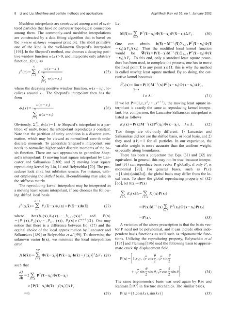
8 Li <strong>and</strong> Liu: <strong>Meshfree</strong> <strong>and</strong> <strong>particle</strong> <strong>methods</strong> <strong>and</strong> <strong>applications</strong> Appl Mech Rev vol 55, no 1, January 2002<br />
<strong>Meshfree</strong> interpolants are constructed among a set of scattered<br />
<strong>particle</strong>s that have no particular topological connection<br />
among them. The commonly-used meshfree interpolations<br />
are constructed by a data fitting algorithm that is based on<br />
the inverse distance weighted principle. The most primitive<br />
one of the kind is the well-known Shepard’s interpolant<br />
194. In the Shepard’s method, one chooses a decaying positive<br />
window function w(x)0, <strong>and</strong> interpolate only arbitrary<br />
function, f (x), as<br />
N<br />
f h x<br />
i1<br />
f i<br />
N<br />
i1<br />
wxx i <br />
wxx i <br />
(25)<br />
where the decaying positive window function, w(xx i ), localizes<br />
around x i . The Shepard’s interpolant then has the<br />
form<br />
i x<br />
N<br />
i1<br />
wxx i<br />
wxx i <br />
(26)<br />
Obviously, N<br />
i1 i (x)1, ie Shepard’s interpolant is a partition<br />
of unity, hence the interpolant reproduces a constant.<br />
Note that the partition of unity condition is a discrete summation,<br />
which may be viewed as normalized zero-th order<br />
discrete moments. To generalize Shepard’s interpolant, one<br />
needs to normalize higher order discrete moments of the basis<br />
function. There are two approaches to generalize Shepard’s<br />
interpolant: 1 moving least square interpolant by Lancaster<br />
<strong>and</strong> Salkauskas 189; <strong>and</strong> 2 moving least square<br />
reproducing kernel by Liu, Li <strong>and</strong> Belytschko 70. The procedures<br />
look alike, but subtleties remain. For instance, without<br />
employing the shifted basis, ill-conditioning may arise in<br />
the stiffness matrix.<br />
The reproducing kernel interpolant may be interpreted as<br />
a moving least square interpolant, if one chooses the following<br />
shifted local basis<br />
n1<br />
f h x,x¯ P i x¯xb i xPx¯xbx¯ (27)<br />
i1<br />
where b(b 1 (x),b 2 (x),¯ ,b n1 (x)) T <strong>and</strong> P(x)<br />
(P 1 (x),P 2 (x),¯ ,P n1 (x)), P i (x)C n1 (). One may<br />
notice that there is a difference between Eq. 27 <strong>and</strong> the<br />
orginal choice of the local approximation by Lancaster <strong>and</strong><br />
Salkauskas 189 or Belytschko et al 59. To determine the<br />
unknown vector b(x), we minimize the local interpolation<br />
error<br />
NP<br />
Jbx¯ x¯x I Px¯x I bx¯ f x I 2 V I (28)<br />
I1<br />
such that<br />
J<br />
b 2 I<br />
P T x¯x I x¯x I <br />
Px¯x I bx¯ f x I V I<br />
0. (29)<br />
Let<br />
Mx¯ª<br />
I<br />
P T x¯x I x¯x I Px¯x I V I . (30)<br />
One can obtain b(x¯)M 1 (x¯) I P T (x¯x I )(x¯<br />
x I )V I f (x I ). Then the modified local kernel function<br />
would be W˜ (x¯)P(x¯x)M 1 (x¯) I P T (x¯x I )(x¯<br />
x I )V I . To this end, only a st<strong>and</strong>ard least square procedure<br />
has been used, to complete the process, one has to move<br />
the fixed point x¯ to any point x; this is why the method<br />
is called moving least square method. By so doing, the corrective<br />
kernel becomes<br />
W˜ Ix limP0M 1 xP T xx I xx I V I ,<br />
x¯→x<br />
I. (31)<br />
If we let P(1,x,x 2 ,¯ ,x n1 ), the moving least square interpolant<br />
is exactly the same as reproducing kernel interpolant.<br />
For comparison, the Lancaster-Salkauskas interpolant is<br />
listed as follows<br />
K I xPxM 1 xP T x I xx I , I. (32)<br />
Two things are obviously different: 1 Lancaster <strong>and</strong><br />
Salkauskas did not use the shifted basis, or local basis, <strong>and</strong> 2<br />
they used V I 1 for all <strong>particle</strong>s. In our experience, the<br />
variable weight is more accurate than the uniform weight,<br />
especially along boundaries.<br />
There has been a conjecture that Eqs. 31 <strong>and</strong> 32 are<br />
equivalent. In general, this may not be true, because interpolant<br />
31 can reproduce basis vector P globally, if only P i is<br />
monomial 70. For general bases, such as P(x)<br />
1,sin(x),sin(2x), the global basis may differ from the local<br />
basis. To show the global reproducing property of 32<br />
66, let f(x)P(x)<br />
K I xf I K I xPx I <br />
I<br />
I<br />
PxM 1 x <br />
I<br />
P T x I xx I Px I <br />
Px. (33)<br />
A variation of the above prescription is that the basis vector<br />
P need not be polynomial, <strong>and</strong> it can include other independent<br />
basis functions as well such as trigonometric functions.<br />
Utilizing the reproducing property, Belytschko et al<br />
195 <strong>and</strong> Fleming 196 used the following basis to approximate<br />
crack tip displacement field,<br />
Px 1,x,y,r cos 2 ,r sin 2<br />
r sin 2 sin ,r cos 2 sin . (34)<br />
The same trigonometric basis was used again by Rao <strong>and</strong><br />
Rahman 197 in fracture mechanics. The similar bases,<br />
Px1,coskx,sinkx (35)